Genetic algorithm

Background

• We want to fit a model with parameters to data
• Given: Data points and a function to calculate a loss function for a given parameter set
• What we don’t have: Derivative of the loss function with respect to the parameters – hence, gradient-descent-type approaches don’t work
• Genetic algorithms are a population-based heuristic method that can optimize even when the loss function is non-differentiable or discontinuous

Example

True model

• We assume a linear model with $n$ data points and $p$ predictors: $$y=X\beta +ϵ,{ϵ}_i\sim \mathcal{N}$$
• The true value of $\beta$ is also sampled from a normal distribution

Optimization algorithm

• We define the residual sum of squares (RSS) as our loss function
• We sample a “population” of $k$ $\beta$ vectors from a normal distribution and store them in a $p\times k$ matrix
• We repeat $m$ times:
  • Selection: The top 50% of individuals (i.e., those with the lowest RSS) are selected and then duplicated to maintain the population size
  • Mutation: We nudge the elements of $P$ by element-wise multiplication with a matrix with identical dimension filled with values sampled from a log-normal distribution with log_mean=0 and log_sd=s
    • all updates maintain the sign of the parameter (=limitation of the algorithm)

Simulate data

set.seed(1)
n <- 5              # number of data points
p <- 3              # number of predictors
beta <- rnorm(p)    
X <- matrix(ncol = p, data = rnorm(n * p))
y <- (X %*% beta)[, 1] + rnorm(n)
dat <- as.data.frame(X)
dat$y <- y

Step by step

# Create parameter population:
k <- 6
P <- matrix(nrow = p, data = rnorm(k * p))

# Predict for first population:
X %*% P[, 1]

           [,1]
[1,] -2.6923821
[2,] -0.9079354
[3,]  2.5717631
[4,] -0.7271242
[5,] -1.9068247

# Predict for all populations:
X %*% P

           [,1]       [,2]       [,3]       [,4]        [,5]        [,6]
[1,] -2.6923821 -0.0364105  1.6766805  3.6372388 -0.75769629  2.55864211
[2,] -0.9079354 -0.1400709 -0.3928391 -1.4049246 -0.08305583 -0.05567578
[3,]  2.5717631 -2.0741455  1.7157369 -0.3375375 -0.25292504  0.25861132
[4,] -0.7271242 -0.6415608  0.7350531  0.1902818 -0.35503138  0.83636691
[5,] -1.9068247  0.3473681 -0.6325051 -0.9800653 -0.11743395  0.18277684

# Residuals for all populations:
X %*% P - y

           [,1]       [,2]       [,3]       [,4]       [,5]       [,6]
[1,] -4.4706386 -1.8146670 -0.1015760  1.8589823 -2.5359527  0.7803857
[2,] -0.2993083  0.4685562  0.2157880 -0.7962975  0.5255712  0.5529513
[3,]  0.8236239 -3.8222847 -0.0324023 -2.0856767 -2.0010643 -1.4895279
[4,] -1.2890299 -1.2034664  0.1731474 -0.3716238 -0.9169370  0.2744612
[5,] -0.6160802  1.6381126  0.6582395  0.3106793  1.1733106  1.4735214

# Define function to calc RSS:
calc_RSS <- function(X, y, P) {
  apply((X %*% P - y)^2, 2, sum)
}

# Calc RSS:
(l <- calc_RSS(X, y, P))

[1] 22.7957041 22.2541658  0.5211913  8.6745785 12.9289711  5.3800447

# determine indices of better half of population:
(ii <- order(l)[1:(k / 2)])

[1] 3 6 4

# select better half and replicate:
(P <- P[, rep(ii, each = 2)])

           [,1]       [,2]       [,3]       [,4]        [,5]        [,6]
[1,]  0.4179416  0.4179416  1.1000254  1.1000254  0.38767161  0.38767161
[2,]  1.3586796  1.3586796  0.7631757  0.7631757 -0.05380504 -0.05380504
[3,] -0.1027877 -0.1027877 -0.1645236 -0.1645236 -1.37705956 -1.37705956

# mutate population:
(P <- P * rlnorm(length(P), sdlog = 0.05))

           [,1]       [,2]       [,3]       [,4]        [,5]        [,6]
[1,]  0.4126804  0.4037936  1.1431183  1.1221411  0.36638711  0.38061849
[2,]  1.4068617  1.3114568  0.7589008  0.7401753 -0.05780171 -0.05106812
[3,] -0.1056888 -0.1046786 -0.1719338 -0.1673538 -1.52039545 -1.41685050

Whole game

Put algorithm in a function

#' Genetic Algorithm Optimizer
#'
#' Implements a genetic algorithm to optimize a parameter matrix for minimizing residual sum of squares (RSS).
#'
#' @param X A matrix of predictor variables.
#' @param y A numeric vector of response values.
#' @param k An integer specifying the number of parameter sets (population size).
#' @param m An integer specifying the number of iterations (default: 1000).
#' @param s A numeric value specifying the standard deviation of the log-normal mutation factor (default: 0.01).
#'
#' @return A list containing:
#' \describe{
#'   \item{P}{A matrix of optimized parameter sets.}
#'   \item{rss_history}{A numeric vector of minimum RSS values across iterations.}
#' }
#'
#' @details
#' This function applies a genetic algorithm to optimize parameters for a given dataset. It initializes a random population of parameters, evaluates the RSS, selects the best-performing half of the population, duplicates them, and applies mutations.
genetic_algorithm_optimizer <- function(X, y, k, 
                                        m = 1000, s = 0.01) {
  P <- matrix(nrow = p, data = rnorm(k * p)) 
  rss_history <- vector(length = m)
  for (i in 1:m) {
    l <- calc_RSS(X, y, P)
    rss_history[i] <- min(l)
    # Selection: Keep the top 50% with lowest RSS and duplicate them
    ii <- rep(order(l)[1:(k / 2)], 2)
    P <- P[, ii]
    # Mutation:
    P <- P * rlnorm(length(P), sdlog = s)
  }
  list(P = P, rss_history = rss_history)
}

Run algorithm

• Some suggestions for playing around with tuning parameters:
  • Vary number of individuals $k$ from 2 to 1000 (only non-odd integers please)
  • Vary number of iterations $m$ from 10 to 1000 (look at plot of RSS to adjust in a smart fashion)
  • Vary standard deviation on log scale of mutation strength $s$ from 0.001 to 0.1

sol <- genetic_algorithm_optimizer(X, y, 
                                   k = 10,
                                   m = 1000, 
                                   s = 0.01)
plot(sol$rss_history, 
     type = 'l', 
     log = 'y', 
     main = 'RSS of "best individual"', 
     ylab = 'RSS on log scale', 
     xlab = 'Iteration')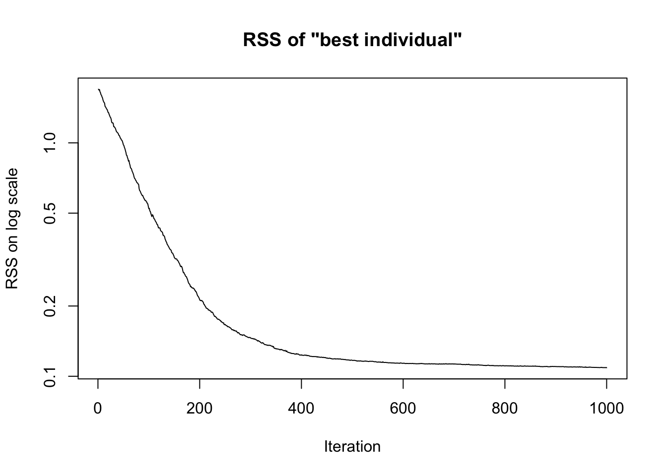

# Comparing the results of linear model solution and genetic algorithm
# when converged, all individuals should be very similar 
# --> showing only individual 1:
data.frame(analytic_solution = coef(lm(y ~ - 1 + ., data = dat)), 
           genetic_algorithm_solution = sol$P[, 1]) 

   analytic_solution genetic_algorithm_solution
V1        0.09093336               -0.005674275
V2        1.23160902                1.175974150
V3       -0.41057390               -0.459881868

• Genetic algorithm seems to have difficulties “finding” solutions with the correct sign of the first element of $\beta$ for small populations – larger populations (e. g. k = 1000) do the job quite reliably