Fitting nonlinear models with stats::nls and nlme::nlme

set.seed(1)
library('tidyverse')

Nonlinear model

n <- 100

pp <- list(
  a = 30,
  b = 2,
  c = 4,
  d = 5
)

dat <- tibble(x = seq(0, 1, length.out = n), 
              y = pp$a * exp(-pp$b * x) + pp$c * x + pp$d + rnorm(n))

dat |> 
  ggplot(aes(x, y)) +
  geom_point()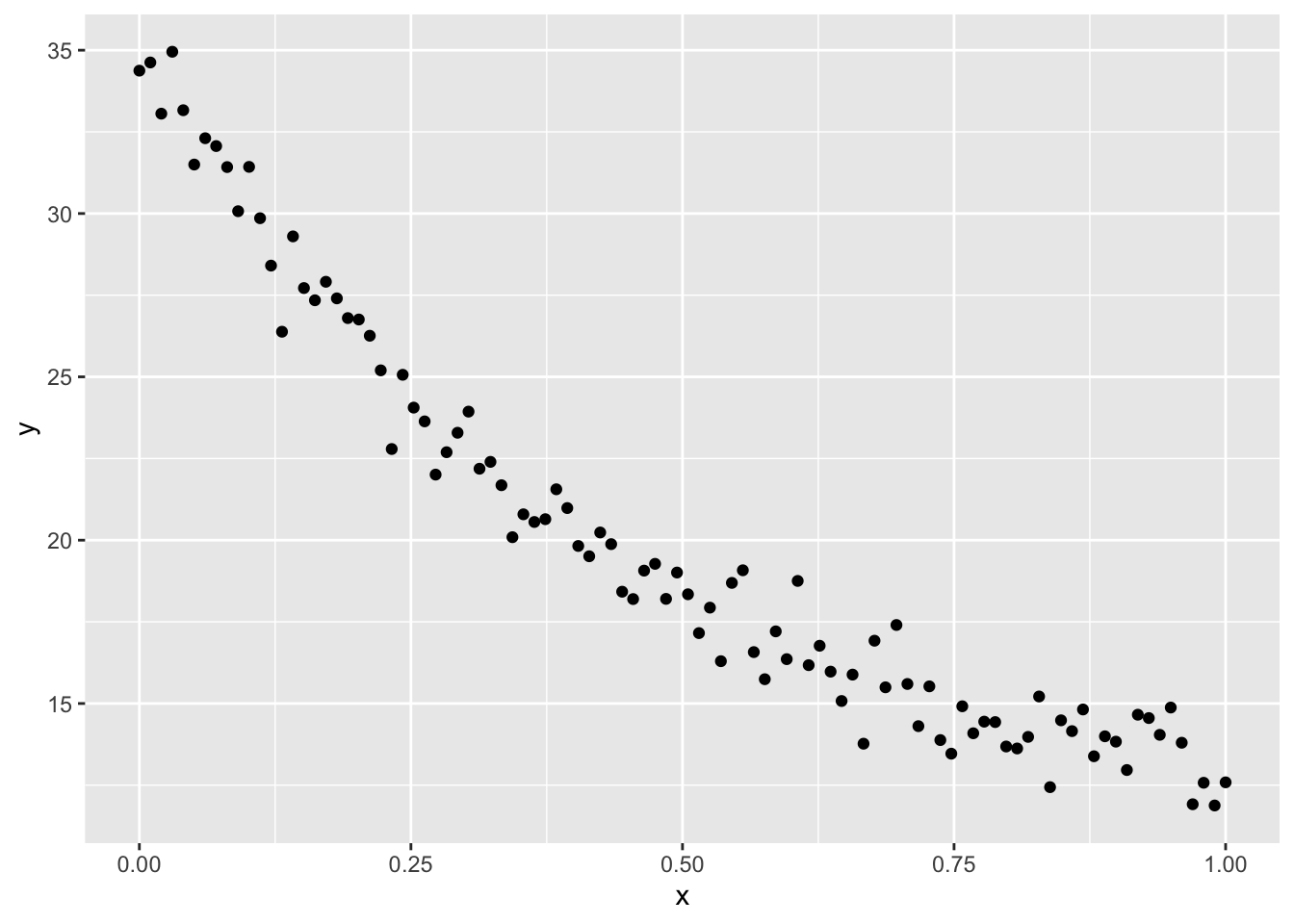

(fm <- nls(y ~ a * exp(-b * x) + c * x + d, 
           data = dat, 
           start = c(a = 1, b = 2, c = 1, d = 1)))

Nonlinear regression model
  model: y ~ a * exp(-b * x) + c * x + d
   data: dat
     a      b      c      d 
26.203  2.234  1.257  8.979 
 residual sum-of-squares: 79.7

Number of iterations to convergence: 11 
Achieved convergence tolerance: 2.134e-06

confint(fm)

Waiting for profiling to be done...

        2.5%     97.5%
a  17.289488 71.226314
b   1.050279  3.484257
c  -6.478915 25.108991
d -36.529815 18.234934

Nonlinear model with mixed effects

library('nlme')

Attaching package: 'nlme'

The following object is masked from 'package:dplyr':

    collapse

pp <- list(
  a = 30,
  b = 2,
  c = 4,
  d = 5
)


nr_of_time_points <- 101
nr_of_individuals <- 100

dat <- tibble(ID = 1:nr_of_individuals,
              a = pp$a + rnorm(nr_of_individuals, sd = 20),
              b = pp$b,
              c = pp$c,
              d = pp$d) |> 
  expand_grid(x = seq(0, 1, length.out = nr_of_time_points)) |> 
  mutate(
    ID_F = factor(paste0('ID', format(ID, justify = 'right'))),
    y = a * exp(-b * x) + c * x + d + rnorm(nr_of_individuals * nr_of_time_points))


dat |> 
  filter(ID <= 10) |> 
  ggplot(aes(x, y, colour = ID_F)) + 
  geom_point()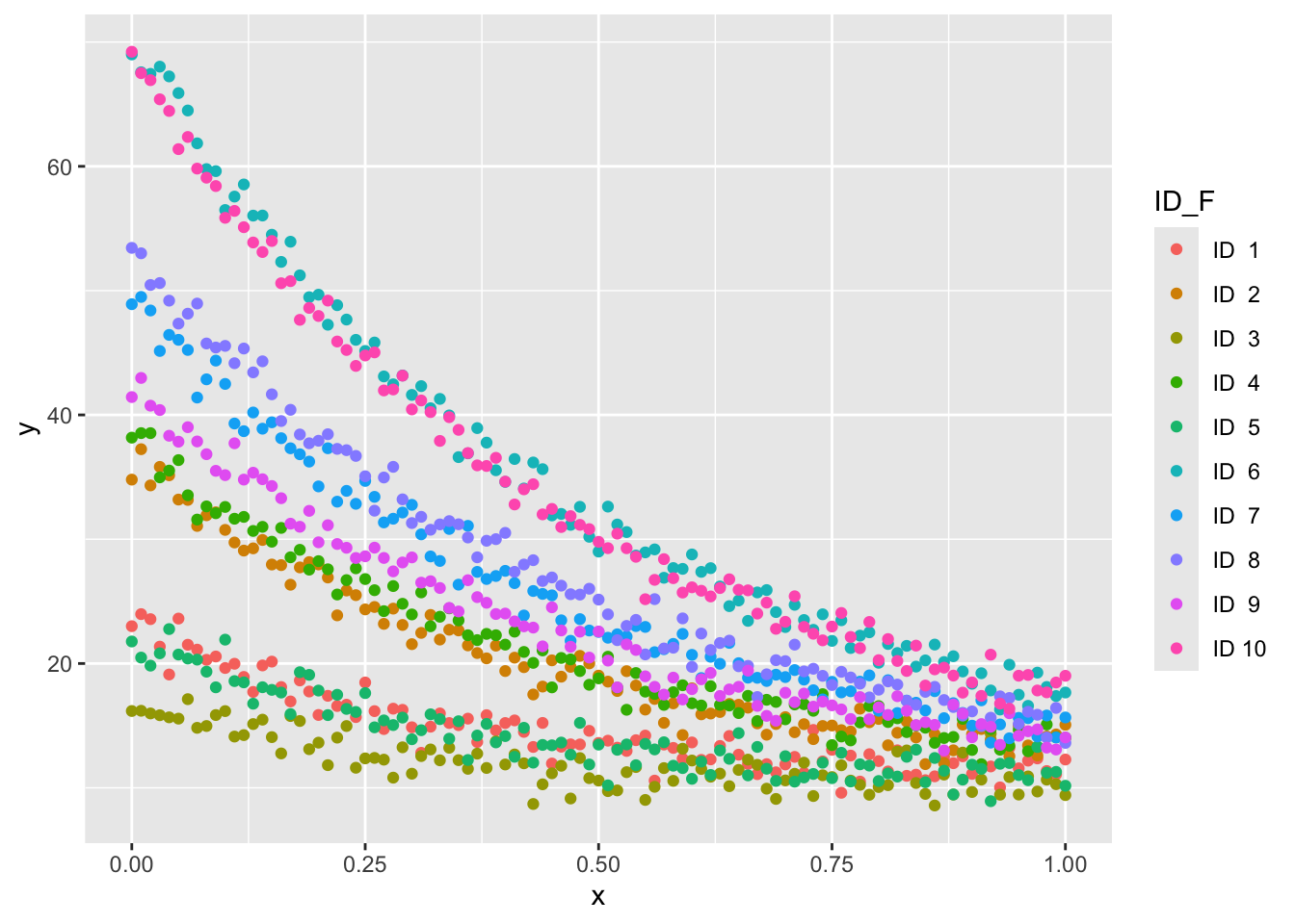

nlme(y ~ a * exp(-b * x) + c * x + d,
     fixed = a + b + c + d ~ 1,
     random = a ~ 1 | ID,
     data = dat,
     start = c(a = 1, b = 2, c = 1, d = 1))

Nonlinear mixed-effects model fit by maximum likelihood
  Model: y ~ a * exp(-b * x) + c * x + d 
  Data: dat 
  Log-likelihood: -14904.82
  Fixed: a + b + c + d ~ 1 
        a         b         c         d 
29.458550  1.998029  4.149341  4.816751 

Random effects:
 Formula: a ~ 1 | ID
               a Residual
StdDev: 19.04709 1.011844

Number of Observations: 10100
Number of Groups: 100