Two-Way-ANOVA with and without interaction vs. individual t-tests

Introduction

Often, the effect of different interventions is to be studied. This can be done by comparing individual sets of interventions (e. g. drug A vs. placebo and drug B vs. placebo) or in a factorial design (e. g. ANOVA). For individual comparisons statistical tests such as the t-test can be appropriate. Importantly, correction for multiple testing should to be carried out. The effect of combination of several drugs can be studied easily in the factorial design, while it is more complicated via t-tests.

Here, it is studied if ANOVA analysis with subsequent joint testing of the relevant hypotheses offers advantages in terms of required sample size / statistical power in comparison to analysis via separate t-tests for some configurations.

set.seed(2)
library('tidyverse')
library('multcomp')
library('knitr')

Simulation model

• Normally distributed data
• Two-way factorial design
  • Factor F1 with levels A and B
  • Factor F2 with levels A and B
• Means:
  • F1 = A, F2 = A → $\mu =0$
  • F1 = A, F2 = B → $\mu =1$
  • F1 = B, F2 = A → $\mu =1$
  • F1 = B, F2 = B → $\mu =3$
• Standard deviation of error:
  • $\sigma =1$
• In treatment coding, this corresponds to the coefficient vector $\beta =(0,1,1,1{)}^T$
• 10 individuals per group

Example of simulated data

generate_data <- function(n = 10, beta = c(0, 1, 1, 1)) {
  dd <- expand_grid(id = 1:n, F1 = c('A', 'B'), F2 = c('A', 'B'))
  X <- model.matrix(~ F1 * F2, data = dd)
  dd |> mutate(y = (X %*% beta)[, 1] + rnorm(nrow(dd)))
}

sample_data <- generate_data()
 
sample_data|> 
  mutate(x = 0) |> 
  ggplot(aes(x, y)) + 
  geom_boxplot() + geom_jitter(width = 0.1, height = 0) +
  facet_wrap(vars(F1, F2), labeller = label_both, ncol = 4) +
  labs(x = '(Points are jittered along x-axis)') +
  theme(axis.text.x=element_blank(),
        axis.ticks.x=element_blank())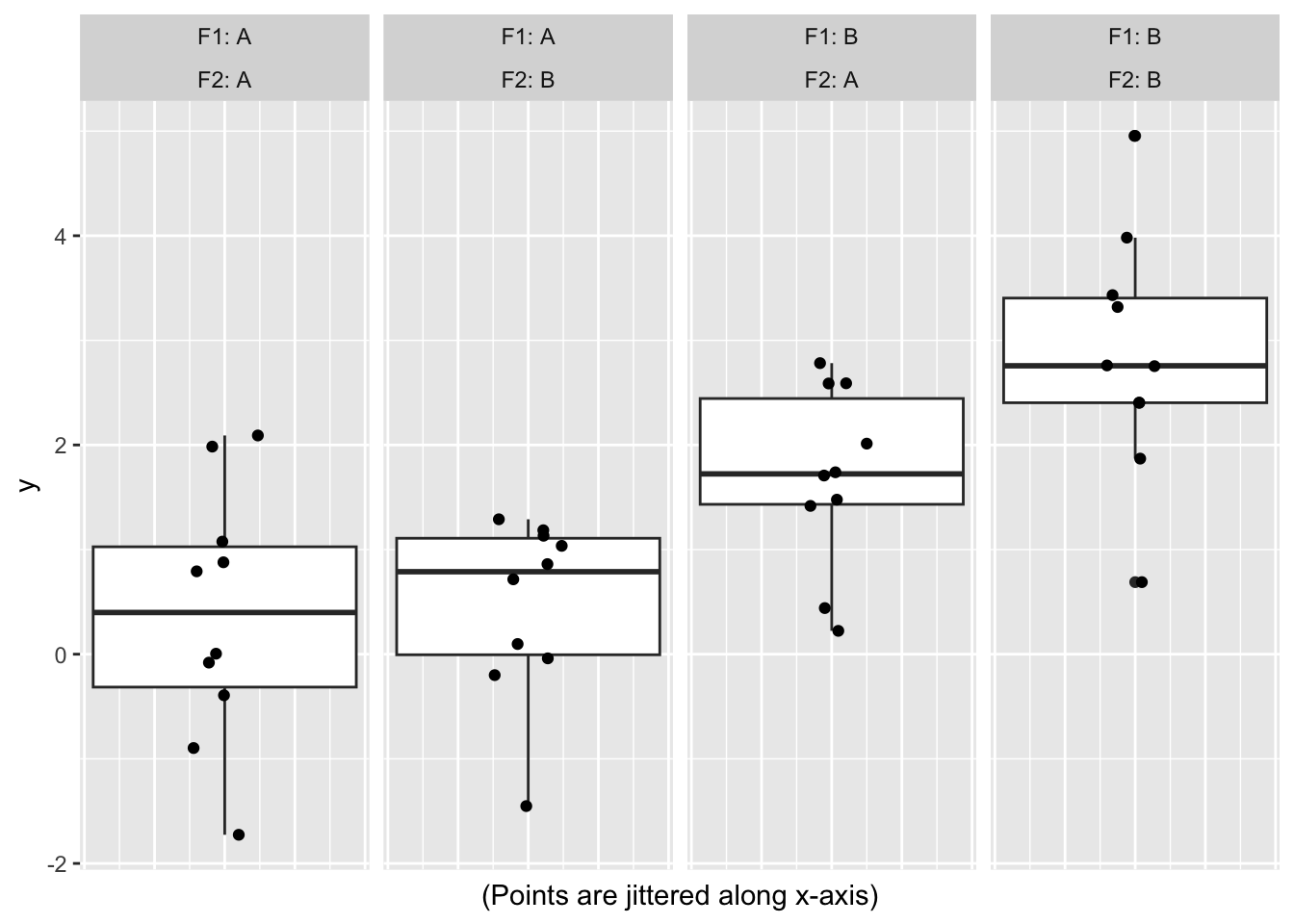

Interaction plots

With base R

with(sample_data, 
     interaction.plot(F1, F2, y))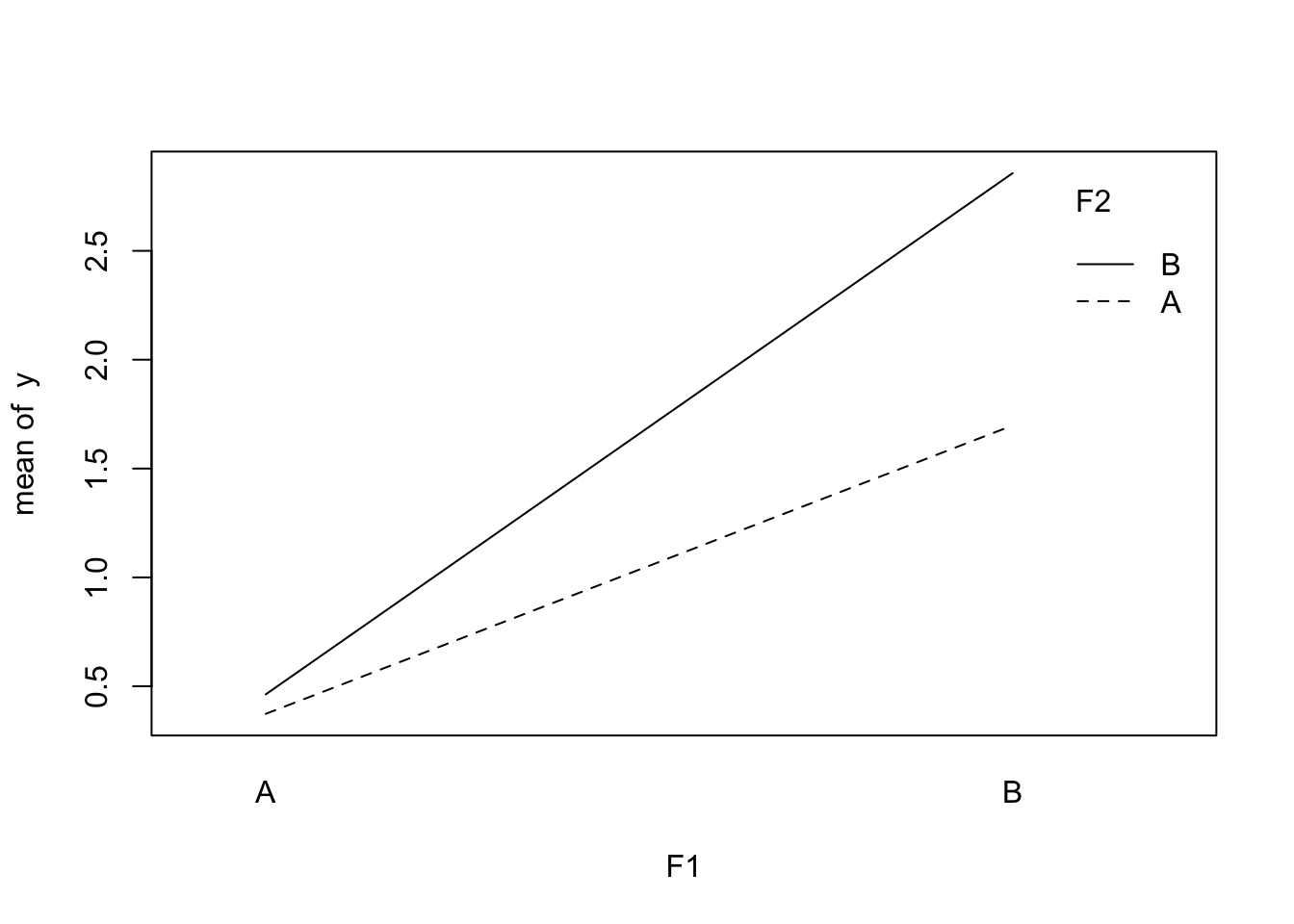

with(sample_data, 
     interaction.plot(F2, F1, y))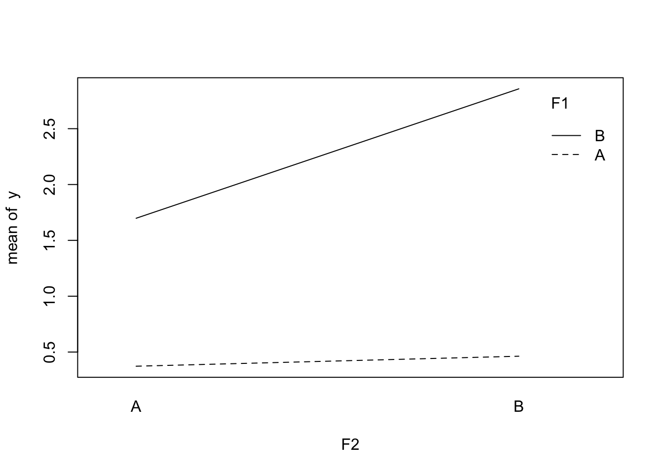

With catstats package

# remotes::install_github("greenwood-stat/catstats")
catstats::intplotarray(y ~ F1 * F2, data = sample_data)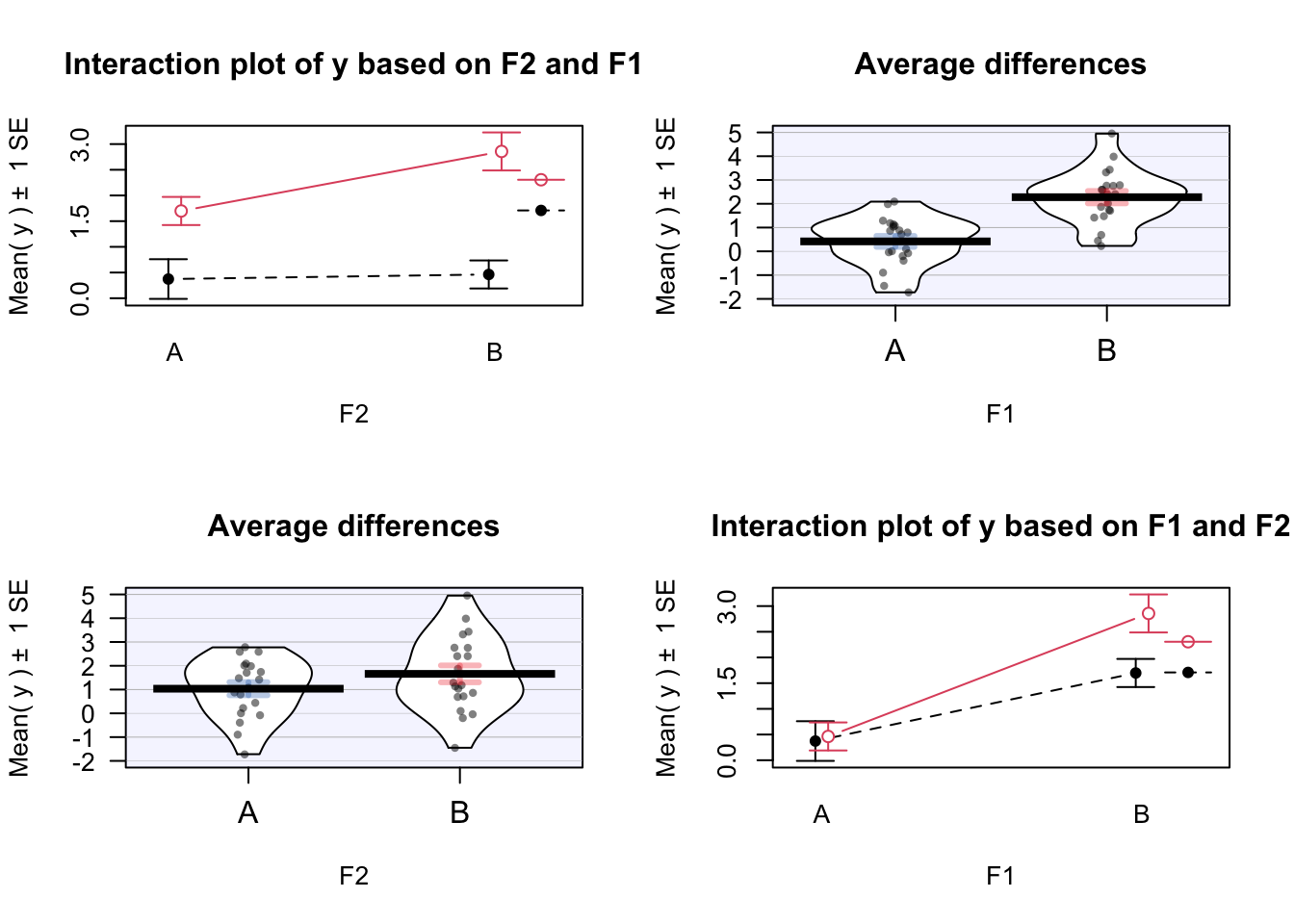

Simulate many datasets in order to estimate power to test the hypotheses

• For ANOVA analysis the multcomp package is used in order to simultaneously test the hypotheses (correction for multiple testing with respect to the two (without interactgion) or three hypotheses (with interaction) is included by design)
• Calculate p-values testing the main effects (${\beta }_1=0$ and ${\beta }_2=0$) and the interaction (${\beta }_3=0$) for each of the simulations
• Estimate power empirically

simulate_two_way_ANOVA <- function(include_interaction = FALSE) {
  if(include_interaction) {
    fm <- lm(y ~ F1 * F2, data = generate_data())
    ii <- -1
  } else {
    fm <- lm(y ~ F1 + F2, data = generate_data(), subset = (F1 == 'A' | F2 == 'A'))
    ii <- c(-1, -4)
  }
  hypotheses_tests <- glht(fm, linfct = paste(names(coef(fm))[ii], '= 0'))
  p_values <- summary(hypotheses_tests)$test$pvalues
  attributes(p_values) <- NULL
  return(p_values)
}

Power of ANOVA analysis without interaction

nr_of_sims <- 1e4
tibble(Effect = c('Main effect 1', 'Main effect 2'),
       Power = rowSums(replicate(n = nr_of_sims, simulate_two_way_ANOVA()) < 
                         0.05) / nr_of_sims) |> 
  kable(align = 'c', digits = 3)

Effect	Power
Main effect 1	0.469
Main effect 2	0.463

Power of ANOVA analysis with interaction

nr_of_sims <- 1e4
tibble(Effect = c('Main effect 1', 'Main effect 2', 'Interaction'),
       Power = rowSums(replicate(n = nr_of_sims, 
                                 simulate_two_way_ANOVA(include_interaction = TRUE)) < 
                         0.05) / nr_of_sims) |> 
  kable(align = 'c', digits = 3)

Effect	Power
Main effect 1	0.438
Main effect 2	0.439
Interaction	0.222

Power of separate t-tests

Bonferroni correction for two tests:

power.t.test(n = 10, delta = 1, sd = 1, sig.level = 0.05 / 2)

     Two-sample t test power calculation 

              n = 10
          delta = 1
             sd = 1
      sig.level = 0.025
          power = 0.4360626
    alternative = two.sided

NOTE: n is number in *each* group

Bonferroni correction for three tests:

• Variance of estimator of interaction effect
  • “the variance of a sum of uncorrelated random variables is equal to the sum of their variances” (Source)
  • Hypothesis for testing main effects: sum with two terms

$$\begin{array}{rl}{H}_0:{\mu }_A-{\mu }_0=0(& ⟺{\beta }_1=0)\\ H_0:{\mu }_B-{\mu }_0=0(& ⟺{\beta }_2=0)\end{array}$$

• Hypotheses for testing interaction: sum with four terms

$$\begin{array}{rl}{H}_0:{\mu }_A+{\mu }_B-{\mu }_{AB}-{\mu }_0=0(& ⟺{\beta }_3=0)\end{array}$$

• Additional formulations of $H_0$ for interaction effect: $$\begin{array}{rlrlrl}{H}_0:& {\mu }_A-{\mu }_0& +& {\mu }_B-{\mu }_0& =& {\mu }_{AB}-{\mu }_0\\ H_0:& {\beta }_1& +& {\beta }_2& =& {\beta }_1+{\beta }_2+{\beta }_3\end{array}$$
• Conclusion: Variance of estimate of interaction effect is twice the variance of the estimate of the main effects

# Main effects:
power.t.test(n = 10, delta = 1, sd = 1, sig.level = 0.05 / 3)

     Two-sample t test power calculation 

              n = 10
          delta = 1
             sd = 1
      sig.level = 0.01666667
          power = 0.3690371
    alternative = two.sided

NOTE: n is number in *each* group

# Interaction effect:
power.t.test(n = 10, delta = 1, sd = sqrt(2), sig.level = 0.05 / 3)

     Two-sample t test power calculation 

              n = 10
          delta = 1
             sd = 1.414214
      sig.level = 0.01666667
          power = 0.1746347
    alternative = two.sided

NOTE: n is number in *each* group

Conclusion

• Power in Two-Way-ANOVA without interaction is slightly greater than power of two separate t-tests corrected with Bonferroni procedure (30 individuals needed in both cases, provided that the control group is ‘recycled’ in the t-test case)
  • Model without interaction:
    • Power for main effects ANOVA: 0.469
    • Power for main effects t-test: 0.436
  • Model with interaction:
    • Power for main effects ANOVA: 0.441
    • Power for main effects t-test: 0.369
    • Power for interaction ANOVA: 0.218
    • Power for interaction t-test: 0.175
• Power in Two-Way-ANOVA with interaction is approximately equal to power of two separate t-tests corrected with Bonferroni procedure (10 additional individuals needed in order to test interaction)
• Power could be improved without increased total sample size by appropriately increasing the size of the control group (not shown here) - see Friedemann’s document (is in local folder however not uploaded)