Kaplan Meier plots

Published

August 3, 2023

Goal: draw facetted Kaplan-Meier-plots with p-value

With ggquickeda

library('tidyverse')

── Attaching core tidyverse packages ──────────────────────── tidyverse 2.0.0 ──
✔ dplyr     1.1.2     ✔ readr     2.1.4
✔ forcats   1.0.0     ✔ stringr   1.5.0
✔ ggplot2   3.4.2     ✔ tibble    3.2.1
✔ lubridate 1.9.2     ✔ tidyr     1.3.0
✔ purrr     1.0.2     
── Conflicts ────────────────────────────────────────── tidyverse_conflicts() ──
✖ dplyr::filter() masks stats::filter()
✖ dplyr::lag()    masks stats::lag()
ℹ Use the conflicted package (<http://conflicted.r-lib.org/>) to force all conflicts to become errors

library('survival')
library('ggquickeda')


Attaching package: 'ggquickeda'

The following object is masked from 'package:base':

    +

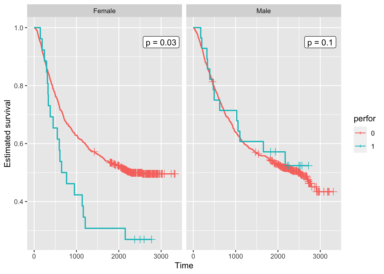
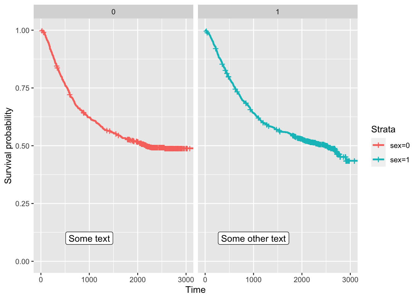
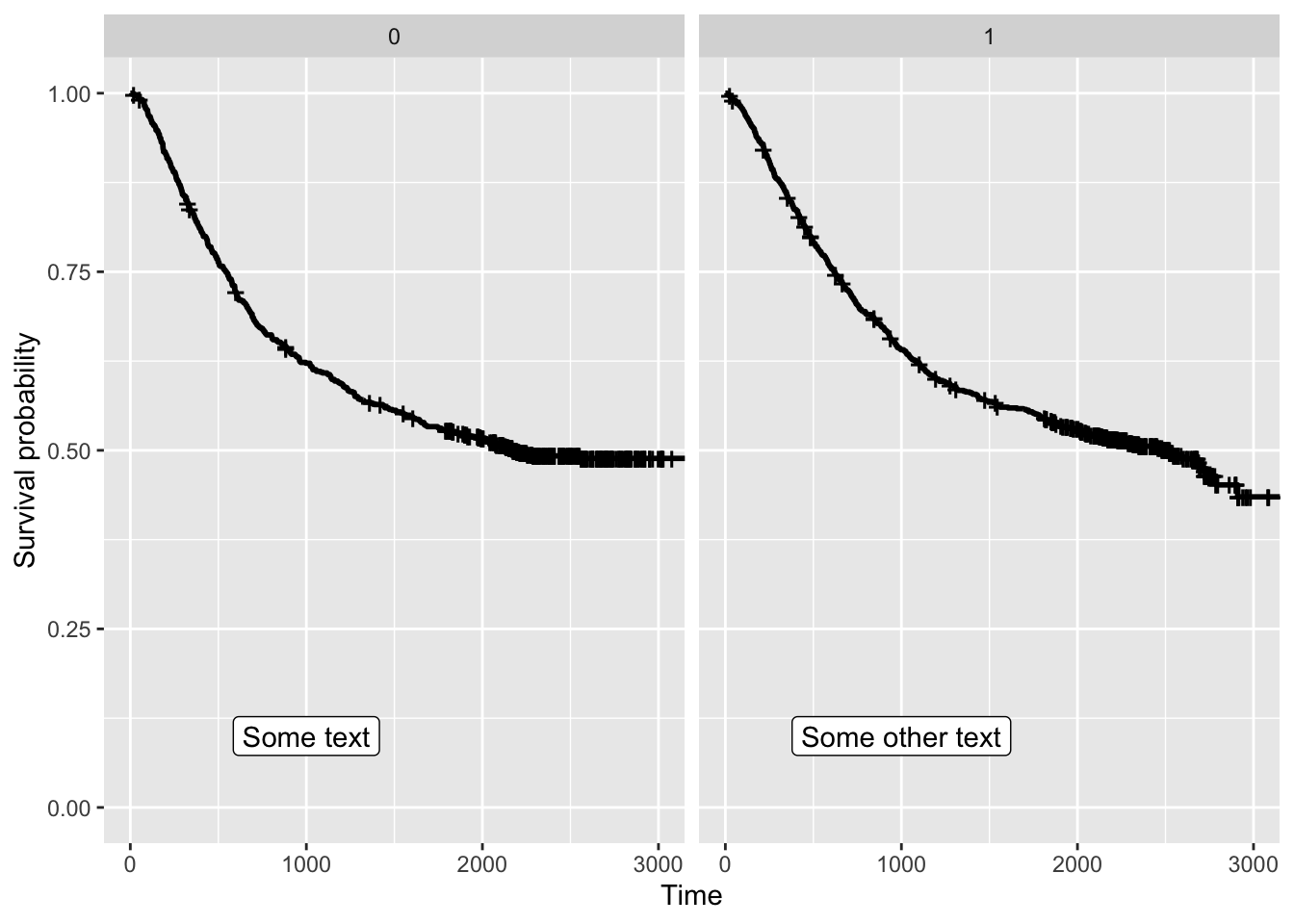
text_to_add <- 
  tribble(~ sex, ~ text, ~ x, ~ y, 
          'Male', 'p = 0.1', 3000, 0.95,
          'Female', 'p = 0.03', 3000, 0.95)



colon |> 
  mutate(sex = case_when(
    sex == 1 ~ 'Male',
    sex == 0 ~ 'Female')) |> 
  mutate(perfor = factor(perfor)) |> 
  
  ggplot(aes(time = time, status = status, colour = perfor)) + 
  facet_wrap(vars(sex)) +
  geom_km() + geom_kmticks() + 
  geom_label(mapping = aes(label = text, 
                           x = x, 
                           y = y), 
             data = text_to_add, 
             inherit.aes = FALSE) +
  labs(x = 'Time', y = 'Estimated survival')

Warning: The following aesthetics were dropped during statistical transformation: status
ℹ This can happen when ggplot fails to infer the correct grouping structure in
  the data.
ℹ Did you forget to specify a `group` aesthetic or to convert a numerical
  variable into a factor?
The following aesthetics were dropped during statistical transformation: status
ℹ This can happen when ggplot fails to infer the correct grouping structure in
  the data.
ℹ Did you forget to specify a `group` aesthetic or to convert a numerical
  variable into a factor?
The following aesthetics were dropped during statistical transformation: status
ℹ This can happen when ggplot fails to infer the correct grouping structure in
  the data.
ℹ Did you forget to specify a `group` aesthetic or to convert a numerical
  variable into a factor?
The following aesthetics were dropped during statistical transformation: status
ℹ This can happen when ggplot fails to infer the correct grouping structure in
  the data.
ℹ Did you forget to specify a `group` aesthetic or to convert a numerical
  variable into a factor?

Warning: Using the `size` aesthetic with geom_path was deprecated in ggplot2 3.4.0.
ℹ Please use the `linewidth` aesthetic instead.

With survminer

Do faceting with survminer

library('survminer')

Loading required package: ggpubr


Attaching package: 'survminer'

The following object is masked from 'package:survival':

    myeloma

fit <- survfit( Surv(time, status) ~ sex + rx, data = colon )
ggsurvplot_facet(fit, colon, facet.by = c('rx', 'perfor'), 
                 pval = TRUE, ggtheme = theme_grey())

Warning: `as.tibble()` was deprecated in tibble 2.0.0.
ℹ Please use `as_tibble()` instead.
ℹ The signature and semantics have changed, see `?as_tibble`.
ℹ The deprecated feature was likely used in the survminer package.
  Please report the issue at <https://github.com/kassambara/survminer/issues>.

Warning: `select_()` was deprecated in dplyr 0.7.0.
ℹ Please use `select()` instead.
ℹ The deprecated feature was likely used in the survminer package.
  Please report the issue at <https://github.com/kassambara/survminer/issues>.

Extract plot object so it can be modified in a more usual ggplot2 style

fit <- survfit( Surv(time, status) ~ sex + rx + perfor, data = colon )
gg <- ggsurvplot(fit, data = colon, color = 'perfor')
gg$plot + theme_grey() + labs(color = 'perfor', x = 'Time [days]') + facet_wrap(~ sex + rx, labeller = label_both)

fit <- survfit( Surv(time, status) ~ sex + perfor, data = colon )
gg <- ggsurvplot(fit, data = colon, color = 'perfor', pval = TRUE, facet.by = 'sex')

Show possible problem in survminer

After facetting, the p-values seem not be correct anymore

fit <- survfit(Surv(time, status) ~ sex + rx, data = colon)
gg <- ggsurvplot(fit, pval = TRUE)
gg

gg$plot + facet_wrap(vars(rx))

gg$plot + facet_wrap(vars(rx, sex))

Try to help someone

Link

library('survival')
library('tidyverse')
library('survminer')

text_to_add <- 
  tribble(~ sex, ~ text, ~ x, ~ y, 
          0, 'Some text', 1000, 0.1,
          1, 'Some other text', 1000, 0.1)

fit <- survfit(Surv(time, status) ~ sex, data = colon)
gg <- ggsurvplot(fit)
gg$plot + facet_wrap(vars(sex)) + theme_gray() + 
  geom_label(aes(x = x, y = y, label = text),
             text_to_add, inherit.aes = FALSE)

gg <- ggsurvplot(fit, palette = c('black', 'black'))
gg$plot + facet_wrap(vars(sex)) + theme_gray() + 
  geom_label(aes(x = x, y = y, label = text),
             text_to_add, inherit.aes = FALSE) +
  theme(legend.position = "none")

With ggsurvfit

Link to package: Link
Link to article: Link
I found this package later – I don’t know why I haven’t across it earlier
At first glance, it seams actively maintained and seems to produce really nice plots

library('ggsurvfit')
glimpse(df_colon)

Rows: 929
Columns: 14
$ id       <dbl> 1, 2, 3, 4, 5, 6, 7, 8, 9, 10, 11, 12, 13, 14, 15, 16, 17, 18…
$ rx       <fct> Levamisole+5-FU, Levamisole+5-FU, Observation, Levamisole+5-F…
$ sex      <fct> Male, Male, Female, Female, Male, Female, Male, Male, Male, F…
$ age      <dbl> 43, 63, 71, 66, 69, 57, 77, 54, 46, 68, 47, 52, 64, 68, 46, 6…
$ obstruct <fct> Not Obstructed, Not Obstructed, Not Obstructed, Obstructed, N…
$ perfor   <dbl> 0, 0, 0, 0, 0, 0, 0, 0, 0, 0, 0, 0, 0, 0, 0, 0, 0, 0, 0, 0, 0…
$ adhere   <fct> Not Adhered, Not Adhered, Adhered, Not Adhered, Not Adhered, …
$ nodes    <dbl> 5, 1, 7, 6, 22, 9, 5, 1, 2, 1, 1, 2, 1, 3, 4, 1, 6, 1, 1, 1, …
$ status   <dbl> 1, 0, 1, 1, 1, 1, 1, 0, 0, 0, 0, 0, 1, 1, 0, 1, 1, 1, 1, 0, 0…
$ differ   <fct> Moderate, Moderate, Moderate, Moderate, Moderate, Moderate, M…
$ extent   <fct> Serosa, Serosa, Muscle, Serosa, Serosa, Serosa, Serosa, Seros…
$ surg     <fct> Limited Time Since Surgery, Limited Time Since Surgery, Limit…
$ node4    <dbl> 1, 0, 1, 1, 1, 1, 1, 0, 0, 0, 0, 0, 0, 0, 0, 0, 1, 0, 0, 0, 0…
$ time     <dbl> 2.6502396, 8.4517454, 1.4839151, 0.6707734, 1.4318960, 2.4750…

survfit2(Surv(time, status) ~ surg, data = df_colon) |>
  ggsurvfit(linewidth = 1) +
  add_confidence_interval() +
  add_risktable() +
  add_quantile(y_value = 0.6, color = "gray50", linewidth = 0.75)

library('tidyverse')
library('survival')
library('tidycmprsk')
library('ggsurvfit')

n <- 100
dat <- tibble(t_death = rexp(n),
              t_relapse = rexp(n),
              t_censoring = rexp(n),
              t_event = pmin(t_death, t_censoring),
              event = ifelse(t_censoring < t_death, 0, 1),
              group = sample(c('Group A', 'Group B'), replace = TRUE, size = 100))

survfit2(Surv(t_event, event) ~ group, data = dat) |> 
  ggsurvfit() + 
  facet_wrap(~ strata) + 
  add_censor_mark()

cuminc(Surv(ttdeath, death_cr) ~ trt + stage, trial) %>%
  ggcuminc(outcome = "death from cancer") + facet_wrap( ~ strata)

survfit2(Surv(time, status) ~ surg, data = df_colon) %>%
  ggsurvfit() +
  add_confidence_interval() +
  facet_wrap(~strata, nrow = 1) +
  theme(legend.position = "none") +
  scale_x_continuous(n.breaks = 6) +
  labs(title = "PFS by Duration between Surgery and Treatment")