The iris dataset

Init

library('tidyverse')
library('lme4')

Data preparation

iris_long <- iris |> 
  mutate(id = 1:nrow(iris)) |> 
  pivot_longer(cols = -c(Species, id), 
               names_to = 'Variable', 
               values_to = 'Value')

Plots

iris_long |> 
  ggplot(aes(Variable, Value, color = Species)) + 
  geom_boxplot()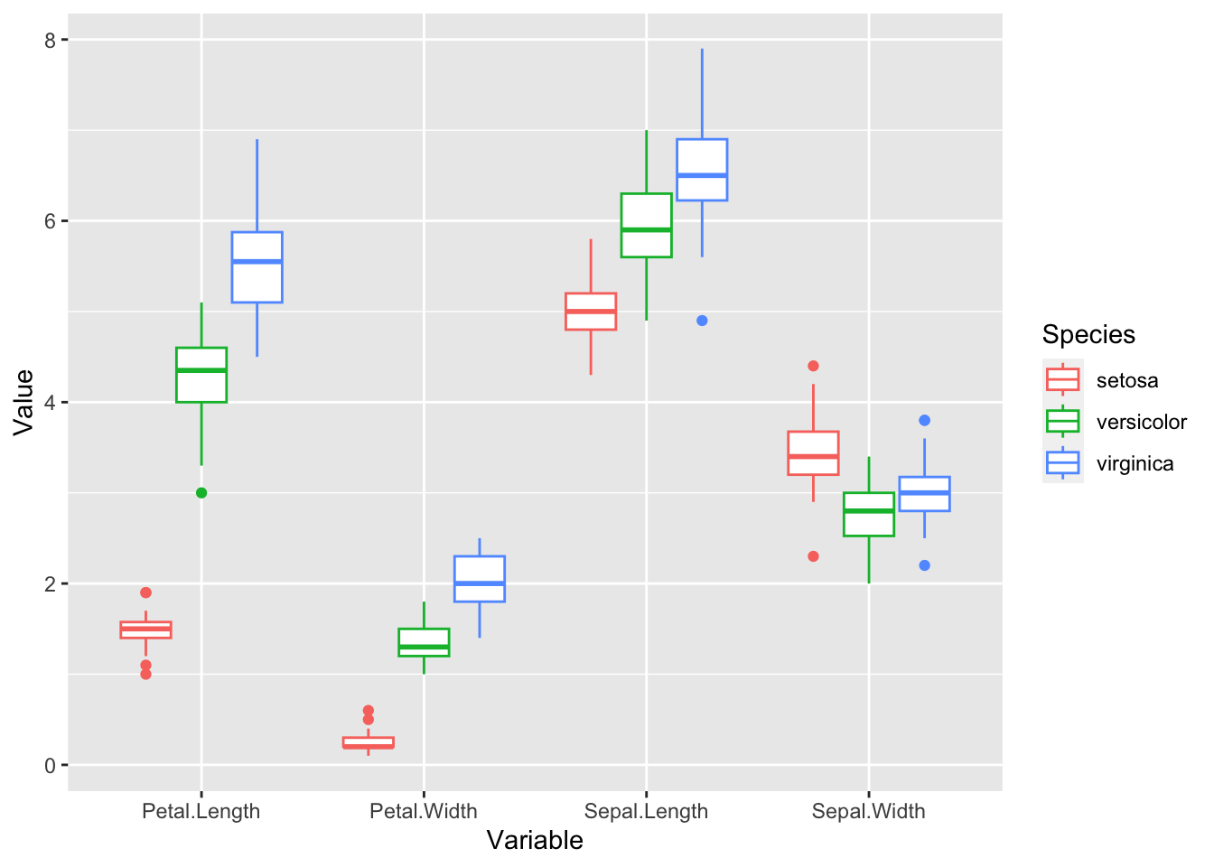

last_plot() + scale_y_log10()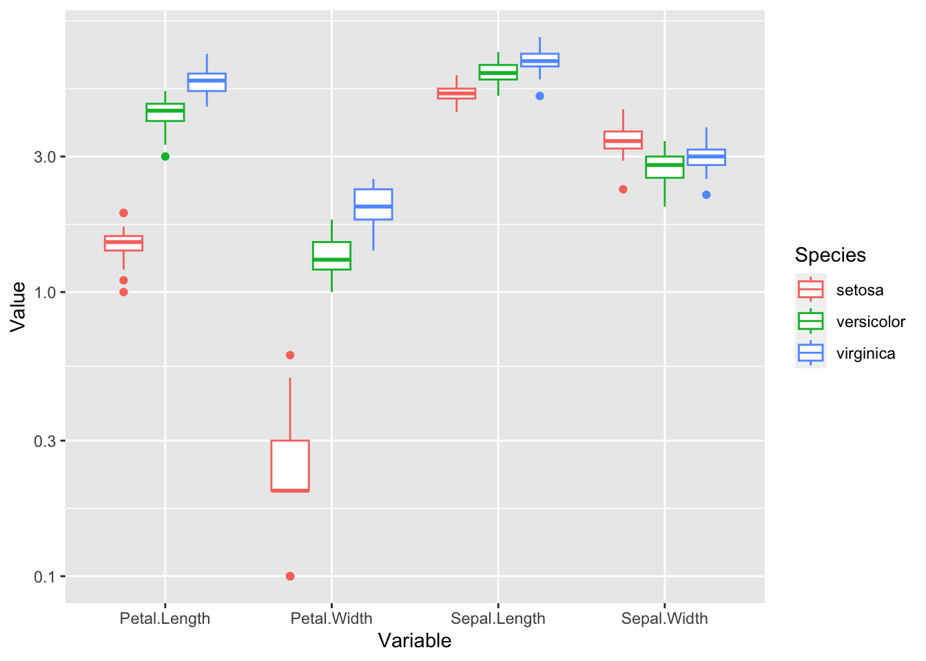 

iris_long |> 
  ggplot(aes(Variable, Value, color = Species)) + 
  geom_jitter(height = 0)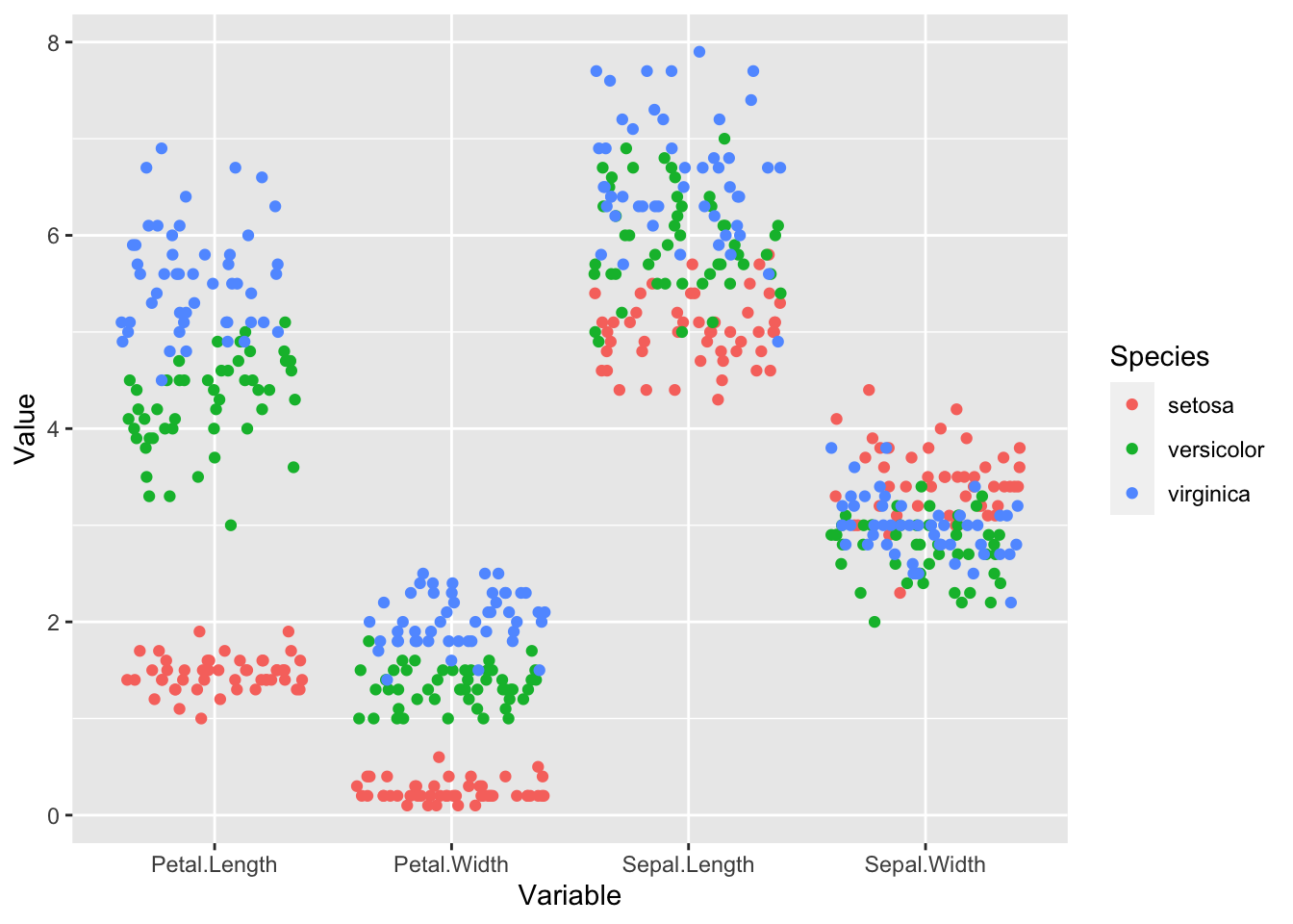

last_plot() + scale_y_log10()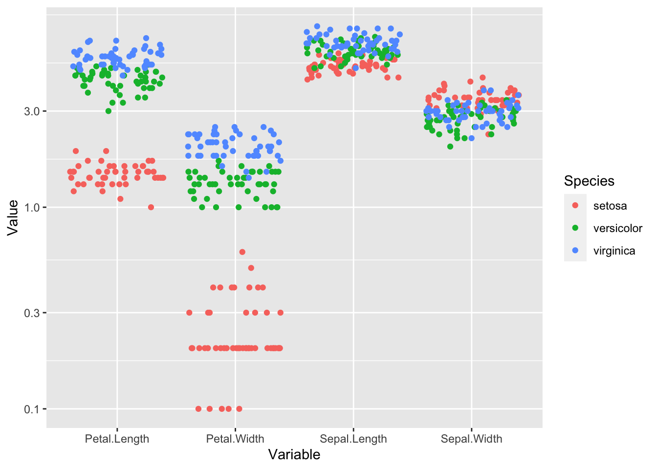 

Models

fitted_model <- 
  lm(Value ~ Species * Variable, 
     data = iris_long)
anova(fitted_model)

Analysis of Variance Table

Response: Value
                  Df  Sum Sq Mean Sq F value    Pr(>F)    
Species            2  309.61  154.80 1019.34 < 2.2e-16 ***
Variable           3 1656.26  552.09 3635.35 < 2.2e-16 ***
Species:Variable   6  282.47   47.08  309.99 < 2.2e-16 ***
Residuals        588   89.30    0.15                      
---
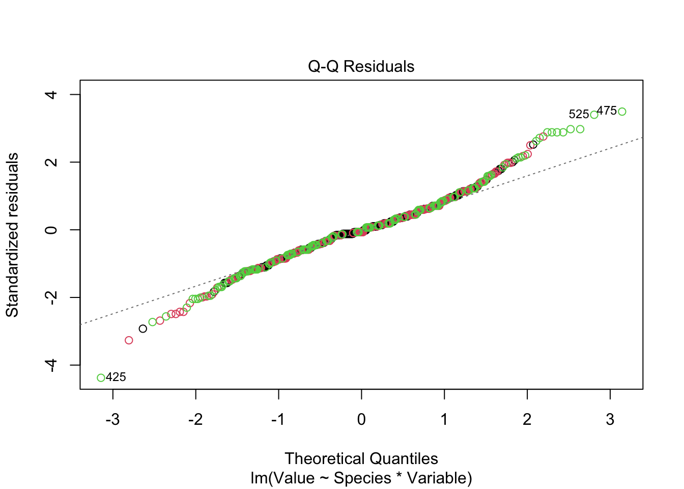
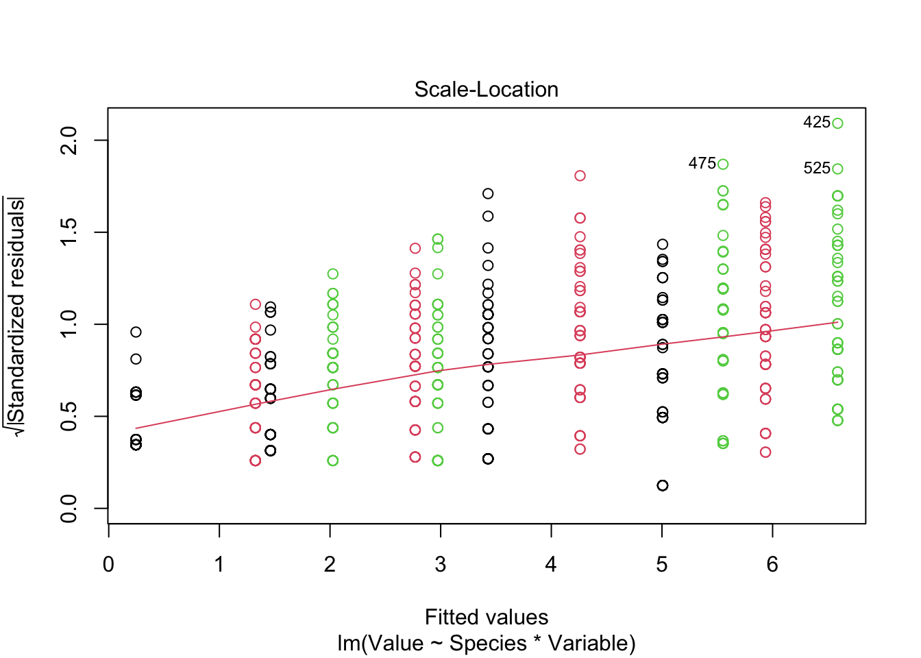
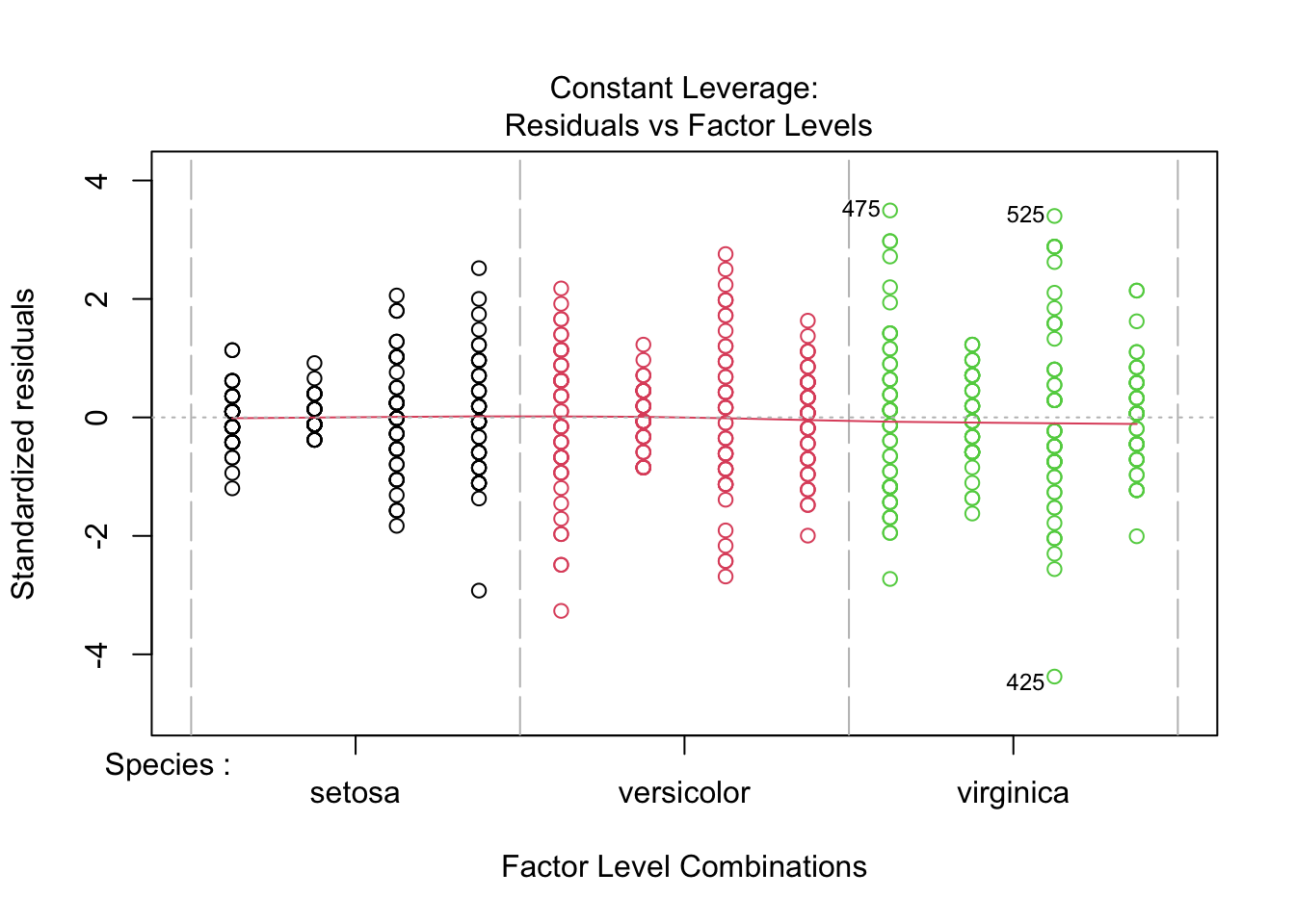
Signif. codes:  0 '***' 0.001 '**' 0.01 '*' 0.05 '.' 0.1 ' ' 1

plot(fitted_model, col = iris_long$Species)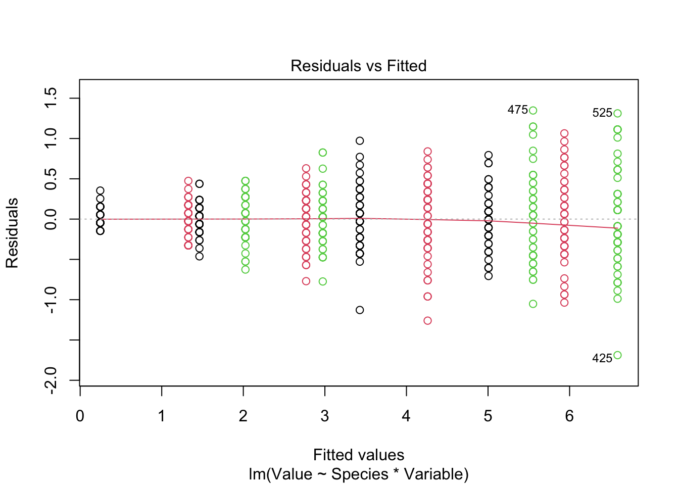

fitted_model <- 
  lm(log(Value) ~ Species * Variable, 
     data = iris_long)
anova(fitted_model)

Analysis of Variance Table

Response: log(Value)
                  Df  Sum Sq Mean Sq F value    Pr(>F)    
Species            2  90.843  45.421 1772.90 < 2.2e-16 ***
Variable           3 297.393  99.131 3869.31 < 2.2e-16 ***
Species:Variable   6  95.977  15.996  624.37 < 2.2e-16 ***
Residuals        588  15.064   0.026                      
---
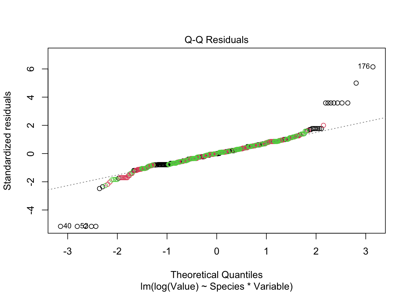
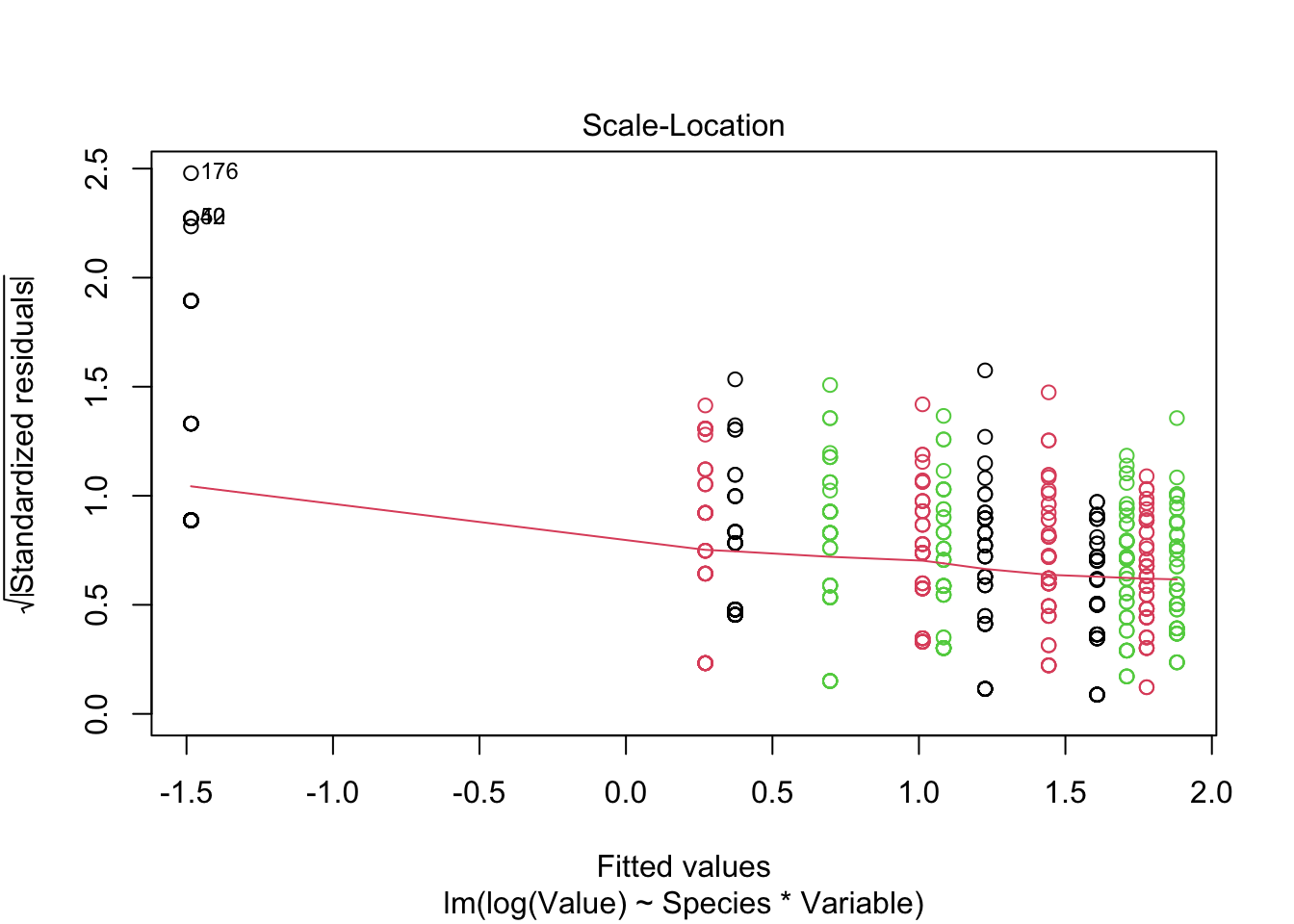
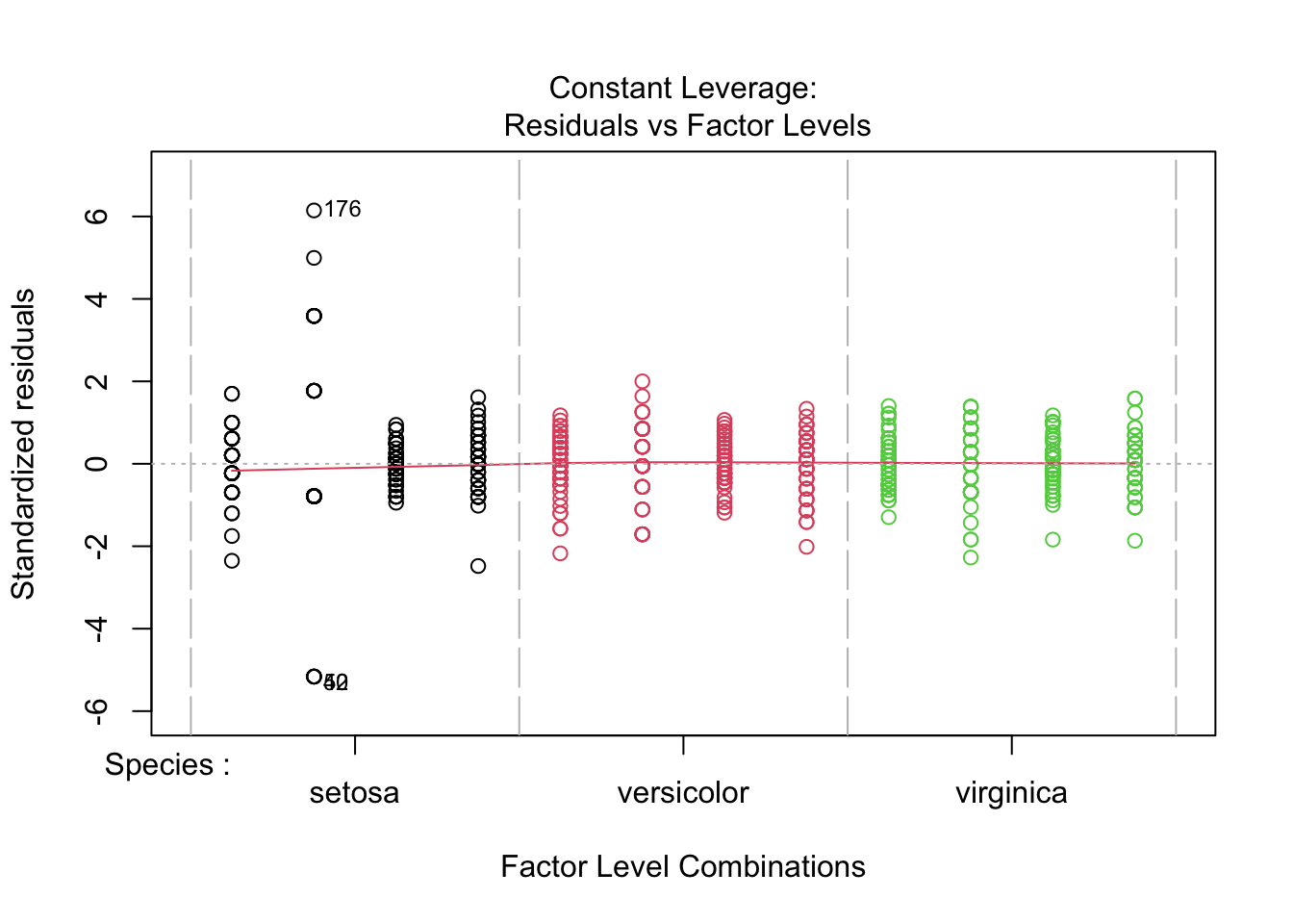
Signif. codes:  0 '***' 0.001 '**' 0.01 '*' 0.05 '.' 0.1 ' ' 1

plot(fitted_model, col = iris_long$Species)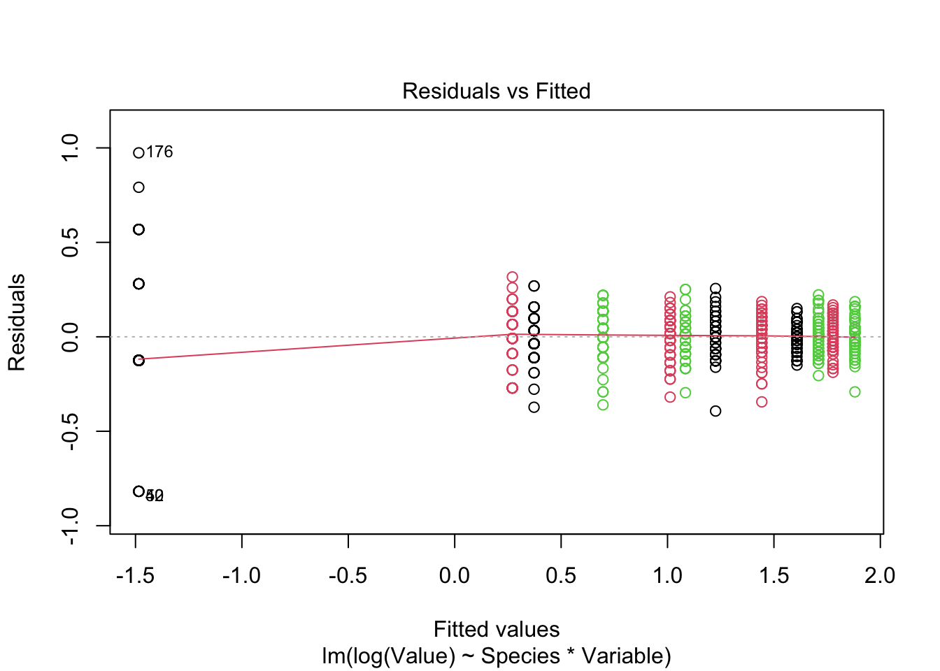

fitted_model <- 
  lmer(log(Value) ~ Species * Variable + (1 | id),
     data = iris_long)
fitted_model

Linear mixed model fit by REML ['lmerMod']
Formula: log(Value) ~ Species * Variable + (1 | id)
   Data: iris_long
REML criterion at convergence: -496.6563
Random effects:
 Groups   Name        Std.Dev.
 id       (Intercept) 0.08565 
 Residual             0.13522 
Number of obs: 600, groups:  id, 150
Fixed Effects:
                           (Intercept)                       Speciesversicolor  
                                0.3728                                  1.0702  
                      Speciesvirginica                     VariablePetal.Width  
                                1.3367                                 -1.8574  
                  VariableSepal.Length                     VariableSepal.Width  
                                1.2354                                  0.8531  
 Speciesversicolor:VariablePetal.Width    Speciesvirginica:VariablePetal.Width  
                                0.6854                                  0.8447  
Speciesversicolor:VariableSepal.Length   Speciesvirginica:VariableSepal.Length  
                               -0.9011                                 -1.0642  
 Speciesversicolor:VariableSepal.Width    Speciesvirginica:VariableSepal.Width  
                               -1.2837                                 -1.4783  

Conclusion

• In general, I like the log scale modeling - however there is a problem with the model on log scale
  • Effects can be given as fold-changes - this seems to make sense to me
  • Species “setosa” is not fitted adequately on log scale - probably measurement error is not adequately modeled on log scale - higher variance of error on log scale
• Dependence on individual level is not considered in the plain linear model
  • Linear mixed model should be considered!!!