import matplotlib.pyplot as plt
import numpy as np
import statsmodels.api as sm
= sm.datasets.statecrime.load_pandas().data
data = data['murder']
murder = data[['poverty', 'hs_grad']].copy()
X 'constant'] = 1
X[
= murder
y = sm.OLS(y, X)
model = model.fit()
results
# Create a plot just for the variable 'Poverty':
= plt.subplots()
fig, ax = sm.graphics.plot_fit(results, 0, ax=ax)
fig "Murder Rate")
ax.set_ylabel("Poverty Level")
ax.set_xlabel("Linear Regression")
ax.set_title(
plt.show()
Exploring the Python library statsmodels
plot_fit
plot_regress_exog
import statsmodels.api as sm
import matplotlib.pyplot as plt
import statsmodels.formula.api as smf
= plt.figure(figsize=(8, 6))
fig = sm.datasets.statecrime.load_pandas()
crime_data = smf.ols('murder ~ hs_grad + urban + poverty + single',
results =crime_data.data).fit()
data'poverty', fig=fig)
sm.graphics.plot_regress_exog(results, plt.show()
plot_partregress
= sm.datasets.statecrime.load_pandas()
crime_data ='murder', exog_i='hs_grad',
sm.graphics.plot_partregress(endog=['urban', 'poverty', 'single'],
exog_others=crime_data.data, obs_labels=False)
data plt.show()
plot_partregress_grid
import matplotlib.pyplot as plt
import statsmodels.api as sm
import statsmodels.formula.api as smf
from statsmodels.graphics.regressionplots import plot_partregress_grid
= plt.figure(figsize=(8, 6))
fig = sm.datasets.statecrime.load_pandas()
crime_data = smf.ols('murder ~ hs_grad + urban + poverty + single',
results =crime_data.data).fit()
data=fig)
plot_partregress_grid(results, fig plt.show()
import statsmodels.api as sm
import pandas
= sm.datasets.get_rdataset("Guerry", "HistData").data
df
= sm.formula.ols('Lottery ~ Literacy + Wealth + C(Region)', data = df).fit()
fm print(fm.summary())
OLS Regression Results
==============================================================================
Dep. Variable: Lottery R-squared: 0.338
Model: OLS Adj. R-squared: 0.287
Method: Least Squares F-statistic: 6.636
Date: Wed, 09 Aug 2023 Prob (F-statistic): 1.07e-05
Time: 13:39:12 Log-Likelihood: -375.30
No. Observations: 85 AIC: 764.6
Df Residuals: 78 BIC: 781.7
Df Model: 6
Covariance Type: nonrobust
==================================================================================
coef std err t P>|t| [0.025 0.975]
----------------------------------------------------------------------------------
Intercept 38.6517 9.456 4.087 0.000 19.826 57.478
C(Region)[T.E] -15.4278 9.727 -1.586 0.117 -34.793 3.938
C(Region)[T.N] -10.0170 9.260 -1.082 0.283 -28.453 8.419
C(Region)[T.S] -4.5483 7.279 -0.625 0.534 -19.039 9.943
C(Region)[T.W] -10.0913 7.196 -1.402 0.165 -24.418 4.235
Literacy -0.1858 0.210 -0.886 0.378 -0.603 0.232
Wealth 0.4515 0.103 4.390 0.000 0.247 0.656
==============================================================================
Omnibus: 3.049 Durbin-Watson: 1.785
Prob(Omnibus): 0.218 Jarque-Bera (JB): 2.694
Skew: -0.340 Prob(JB): 0.260
Kurtosis: 2.454 Cond. No. 371.
==============================================================================
Notes:
[1] Standard Errors assume that the covariance matrix of the errors is correctly specified.
= sm.graphics.influence_plot(fm, criterion="cooks")
fig fig.show()
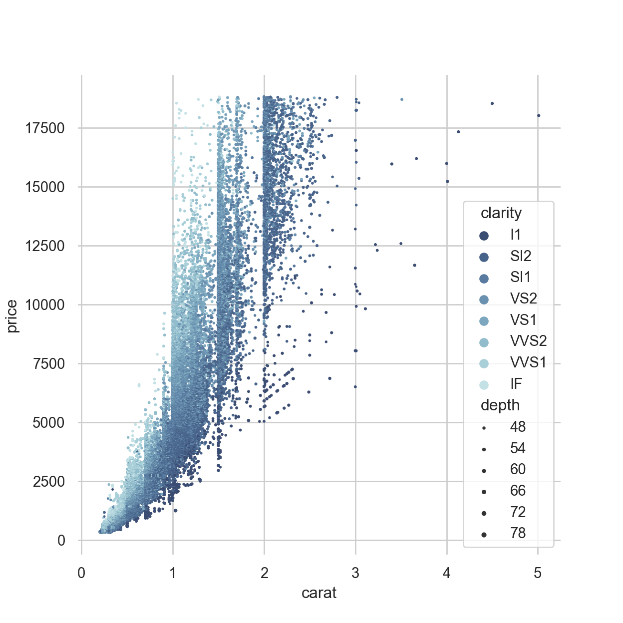
import seaborn as sns
import matplotlib.pyplot as plt
="whitegrid")
sns.set_theme(style
# Load the example diamonds dataset
= sns.load_dataset("diamonds")
diamonds
# Draw a scatter plot while assigning point colors and sizes to different
# variables in the dataset
= plt.subplots(figsize=(6.5, 6.5))
f, ax =True, bottom=True)
sns.despine(f, left= ["I1", "SI2", "SI1", "VS2", "VS1", "VVS2", "VVS1", "IF"]
clarity_ranking ="carat", y="price",
sns.scatterplot(x="clarity", size="depth",
hue="ch:r=-.2,d=.3_r",
palette=clarity_ranking,
hue_order=(1, 8), linewidth=0,
sizes=diamonds, ax=ax) data