Simulate time to-event-data

Intro

In this post, two methods to draw from a survival time distribution defined by an arbitrary hazard function are demonstrated. First, some central equations of survival analysis are given in order to refresh the background and establish a consistent notation. Then, the two different approaches are demonstrated.

Mathematical aspects

• Taken from wikipedia - at this wikipedia page also further explanation can be found
• Survival function $S$ $$S(t)=Pr(T>t)$$
• Hazard function $\lambda$ $$\lambda (t)=-S^{\prime }(t)/S(t)$$
• Cumulative hazard function $\mathrm{\Lambda }$ $$\mathrm{\Lambda }(t)={\int }_0^t\lambda (u)du$$
• Relation between $\mathrm{\Lambda }$ and $S$ $$S(t)=exp(-\mathrm{\Lambda }(t))$$

Ad hoc code to draw from survival time distribution

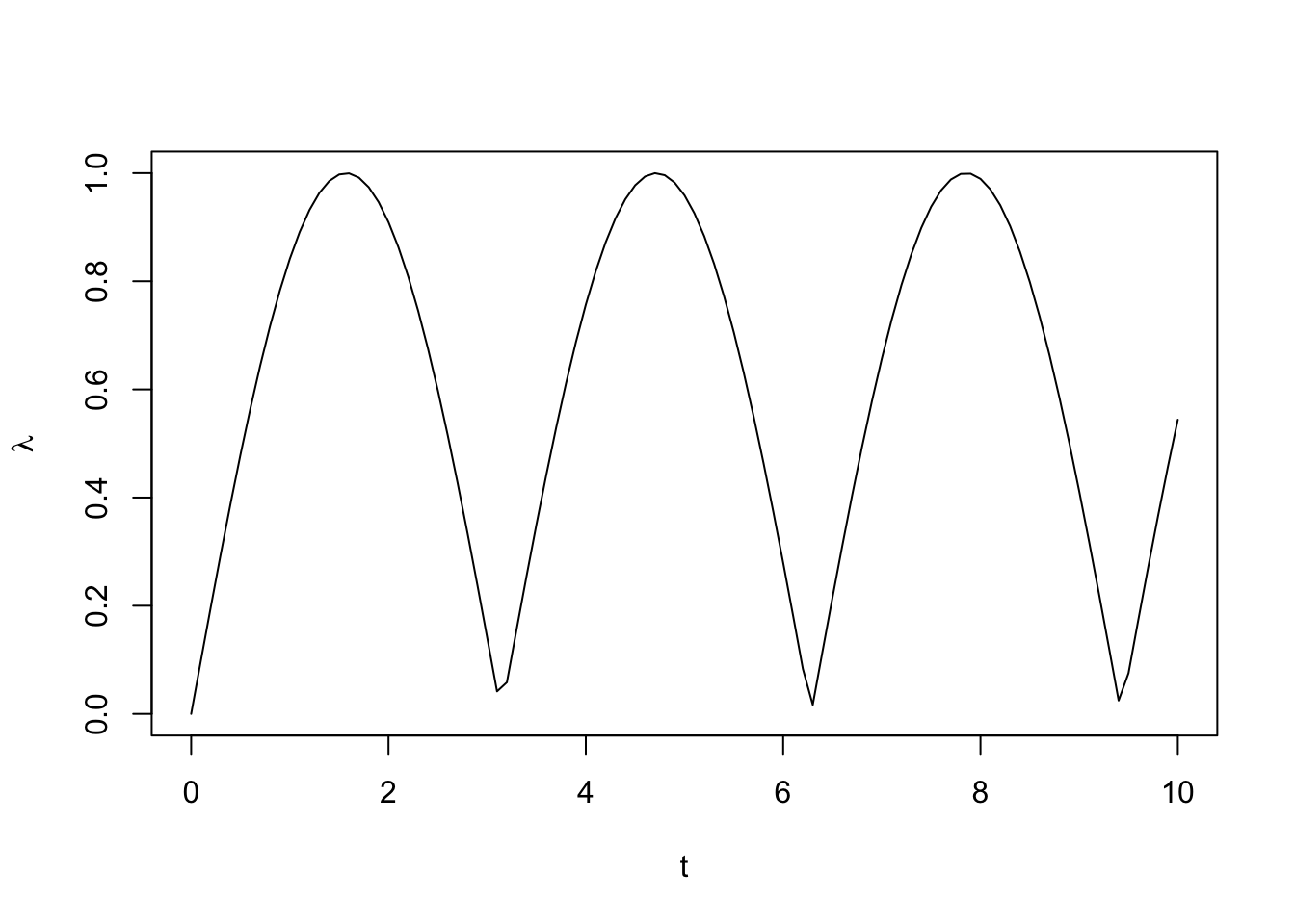
set.seed(1)
library('survival')

# define hazard function:
lambda <- function(t) {
  abs(sin(t))
}


# hazard for t = 7 and t = 12:
lambda(c(7, 12)) 

[1] 0.6569866 0.5365729

# plot hazard function:
plot(lambda, from = 0, to = 10, xlab = 't', ylab = expression(lambda))

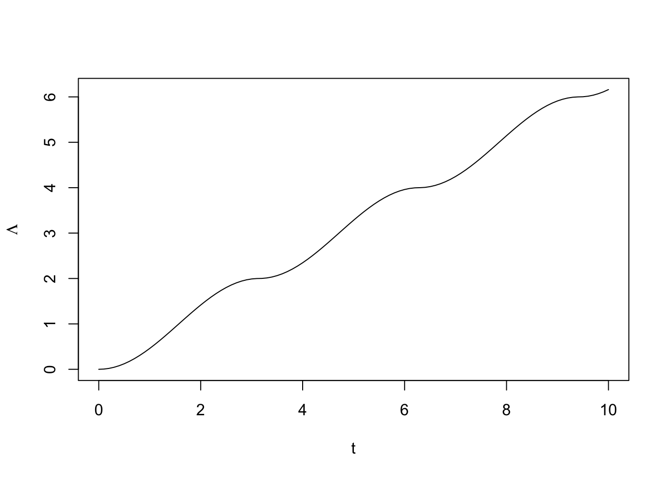
# define function that computes cumulative hazard function:
Lambda <- Vectorize(
  function(t) {
    integrate(lambda,
              subdivisions = 1e3L,
              lower = 0, 
              upper = t)$value
  })

# cumulative hazard for t = 3
Lambda(3) 

[1] 1.989992

# plot cumulative hazard function:
plot(Lambda, from = 0, to = 10, xlab = 't', ylab = expression(Lambda))

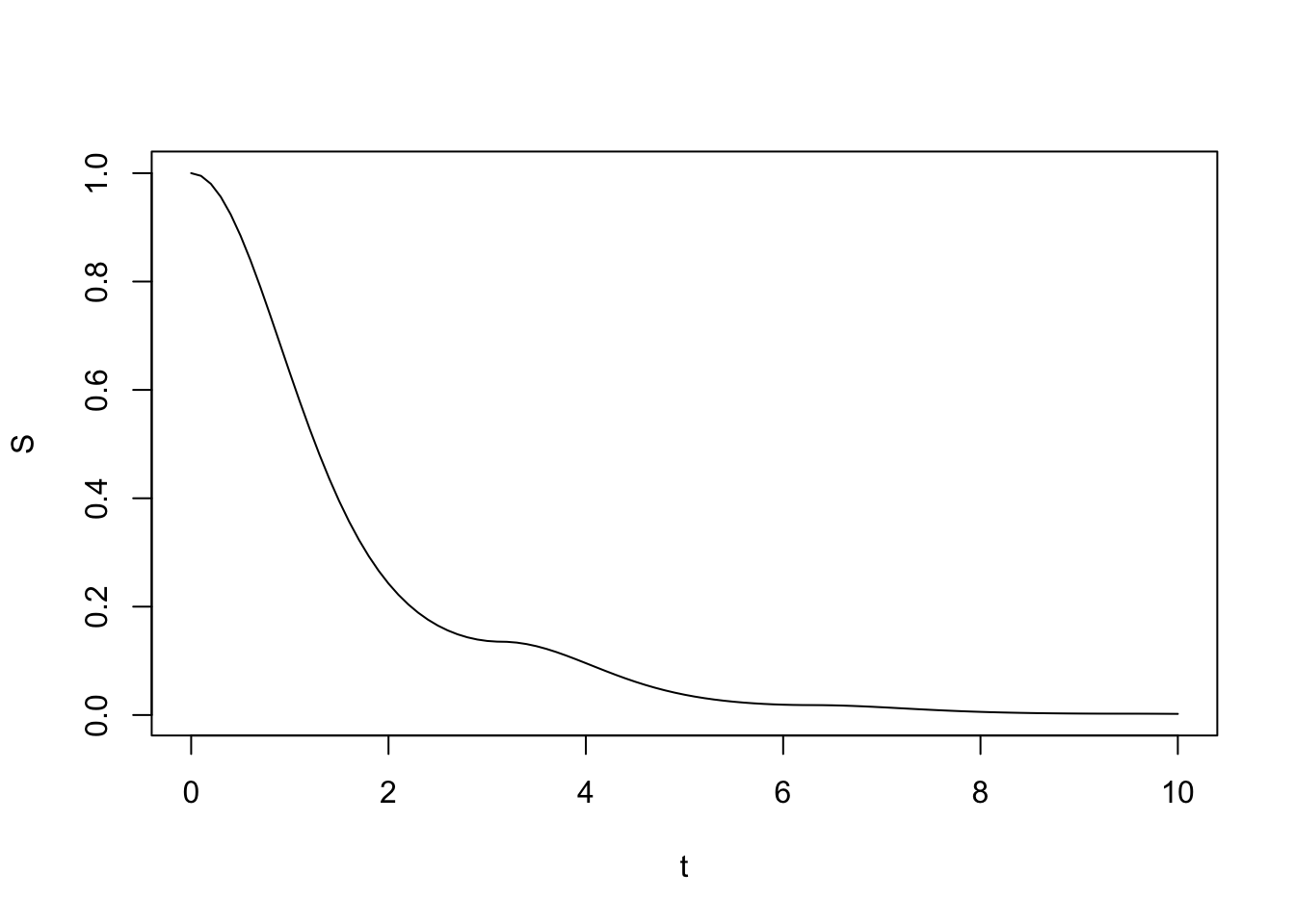
# define function that computes survival function 
# from cumulative hazard function:
S <- Vectorize(
  function(t) {
    exp(-Lambda(t))
  })

# plot survival function:
plot(S, from = 0, to = 10, xlab = 't')

# determine at which time cumulative hazard
# reaches 2e1 (i. e. S(t) < 1e-8)
# the value is used as upper bound for
# optimization to find the quantile
upper_bound <- optimize(
  function(x) {
    abs(Lambda(x) - 2e1)
  }, 
  interval = c(0, 1e2))$minimum

# define function to compute quantile of survival function
quantile_function <- Vectorize(
  function(t) {
    optimize(function(x) {
      abs(S(x) - t)}, 
      interval = c(0, upper_bound))$min
  })

# compute some quantiles for hazard function
# that has been specified above:
quantile_function(c(0.25, 0.5, 0.75))

[1] 1.9674130 1.2589101 0.7779829

# evaluate how long it takes to determine 10 quantiles:
microbenchmark::microbenchmark(quantile_function(1:10))

Warning in microbenchmark::microbenchmark(quantile_function(1:10)): less
accurate nanosecond times to avoid potential integer overflows

Unit: milliseconds
                    expr      min       lq     mean   median       uq      max
 quantile_function(1:10) 10.19416 10.70949 11.62673 11.01805 12.94298 15.45019
 neval
   100

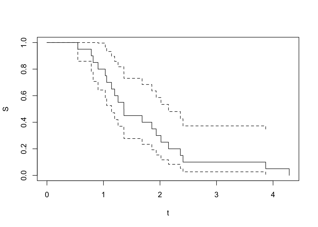
# draw n random numbers from survival distribution 
# defined by hazard function above
(times <- quantile_function(runif(n = 20)))

 [1] 0.9040743 1.0566904 2.0173300 1.9328205 0.8170795 1.3620799 2.4072092
 [8] 0.7842570 3.8702329 0.5462974 1.0317729 1.1427625 1.6834271 1.3608340
[15] 1.2579906 2.3602768 1.1977742 4.2861974 1.8556640 2.1505993

plot(survfit(Surv(times) ~ 1), xlab = 't', ylab = 'S')

More sophisticated solution using the coxed package

• Solution found here:

library('coxed')

my.hazard <- function(t){ 
  abs(sin(t)) * 0.01
}

simdata <- sim.survdata(N = 100, 
                        T = 1000, 
                        hazard.fun = my.hazard)

Warning in FUN(X[[i]], ...): 0 additional observations right-censored because the user-supplied hazard function
                                  is nonzero at the latest timepoint. To avoid these extra censored observations, increase T

plot(survfit(Surv(simdata$data$y) ~ 1), xlab = 't', ylab = 'S')

Conclusion

It is possible to draw survival times defined by an arbitrary hazard function with just a few lines of code. However, the code is not very time-efficient and there might be issues with numerical stability in certain constellations - hence, plausibility of the results needs to be checked manually.

The coxed package provides convenient, more sophisticated methods to achieve a similar goal. However, the coxed approach might be more difficult to adapt to specific situations since the code base is more rigid.