library(survival)
library(mstate)
tmat <- transMat(list(c(2,3,4), c(3,4), c(4), c()), c('tox', 'twist', 'rel', 'death'))

data <- data.frame(id = c(1, 1, 1, 1, 1, 2, 2, 2, 2, 2, 1, 2, 3, 3, 3, 4, 4, 4, 5, 5, 5),
                   from = c(1, 1, 1, 2, 2, 1, 1, 1, 2, 2, 3, 3, 1, 1, 1, 1, 1, 1, 1, 1, 1),
                   to = c(2, 3, 4, 3, 4, 2, 3, 4, 3, 4, 4, 4, 2, 3, 4, 2, 3, 4, 2, 3, 4),
                   start_time = c(0, 0, 0, 5, 5, 0, 0, 0, 4, 4, 8, 9, 0, 0, 0, 0 , 0 , 0, 0, 0, 0),
                   stop_time = c(5, 5, 5, 8, 8, 4, 4, 4, 9, 9, 12, 13, 2, 2, 2, 3, 3, 3, 7, 7, 7),
                   status = c(1, 0, 0, 0, 1, 1, 0 , 0 , 0, 1, 0, 0, 0 , 0, 1, 0 , 1, 0, 0 , 0 , 0),
                   group = c('a', 'a', 'a', 'a', 'a', 'b', 'b', 'b', 'b', 'b', 'a', 'b', 'a', 'a', 'a', 'b', 'b', 'b', 'b', 'b', 'b'))
data$trans <- data$to - 1

fm <- coxph(Surv(time = start_time, time2 = stop_time, event = status) ~ strata(trans), data = data)

fm_msfit <- msfit(object = fm, trans = tmat)
plot(fm_msfit)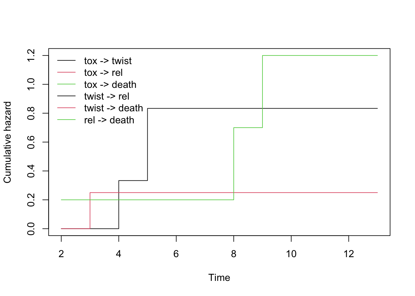
p_model <- probtrans(fm_msfit, predt = 0)
p_model
[[1]]
time pstate1 pstate2 pstate3 pstate4 se1 se2 se3 se4
1 0 1.00 0.0 0.0 0.00 0.00000000 0.0000000 0.0000000 0.0000000
2 2 0.80 0.0 0.0 0.20 0.16000000 0.0000000 0.0000000 0.1600000
3 3 0.60 0.0 0.2 0.20 0.19209373 0.0000000 0.1552417 0.1600000
4 4 0.40 0.2 0.2 0.20 0.18487233 0.1479114 0.1552417 0.1600000
5 5 0.20 0.4 0.2 0.20 0.13617799 0.1756259 0.1552417 0.1600000
6 8 0.10 0.4 0.2 0.30 0.08447551 0.1756259 0.1552417 0.1622840
7 9 0.05 0.4 0.2 0.35 0.04908185 0.1756259 0.1552417 0.1663768
8 13 0.05 0.4 0.2 0.35 0.04908185 0.1756259 0.1552417 0.1663768
[[2]]
time pstate1 pstate2 pstate3 pstate4 se1 se2 se3 se4
1 0 0 1 0 0 0 0 0 0
2 2 0 1 0 0 0 0 0 0
3 3 0 1 0 0 0 0 0 0
4 4 0 1 0 0 0 0 0 0
5 5 0 1 0 0 0 0 0 0
6 8 0 1 0 0 0 0 0 0
7 9 0 1 0 0 0 0 0 0
8 13 0 1 0 0 0 0 0 0
[[3]]
time pstate1 pstate2 pstate3 pstate4 se1 se2 se3 se4
1 0 0 0 1 0 0 0 0 0
2 2 0 0 1 0 0 0 0 0
3 3 0 0 1 0 0 0 0 0
4 4 0 0 1 0 0 0 0 0
5 5 0 0 1 0 0 0 0 0
6 8 0 0 1 0 0 0 0 0
7 9 0 0 1 0 0 0 0 0
8 13 0 0 1 0 0 0 0 0
[[4]]
time pstate1 pstate2 pstate3 pstate4 se1 se2 se3 se4
1 0 0 0 0 1 0 0 0 0
2 2 0 0 0 1 0 0 0 0
3 3 0 0 0 1 0 0 0 0
4 4 0 0 0 1 0 0 0 0
5 5 0 0 0 1 0 0 0 0
6 8 0 0 0 1 0 0 0 0
7 9 0 0 0 1 0 0 0 0
8 13 0 0 0 1 0 0 0 0
$trans
to
from tox twist rel death
tox NA 1 2 3
twist NA NA 4 5
rel NA NA NA 6
death NA NA NA NA
$method
[1] "aalen"
$predt
[1] 0
$direction
[1] "forward"
attr(,"class")
[1] "probtrans"plot(p_model, use.ggplot = TRUE)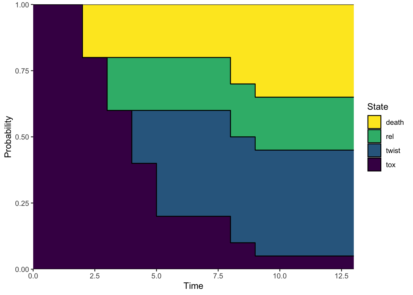
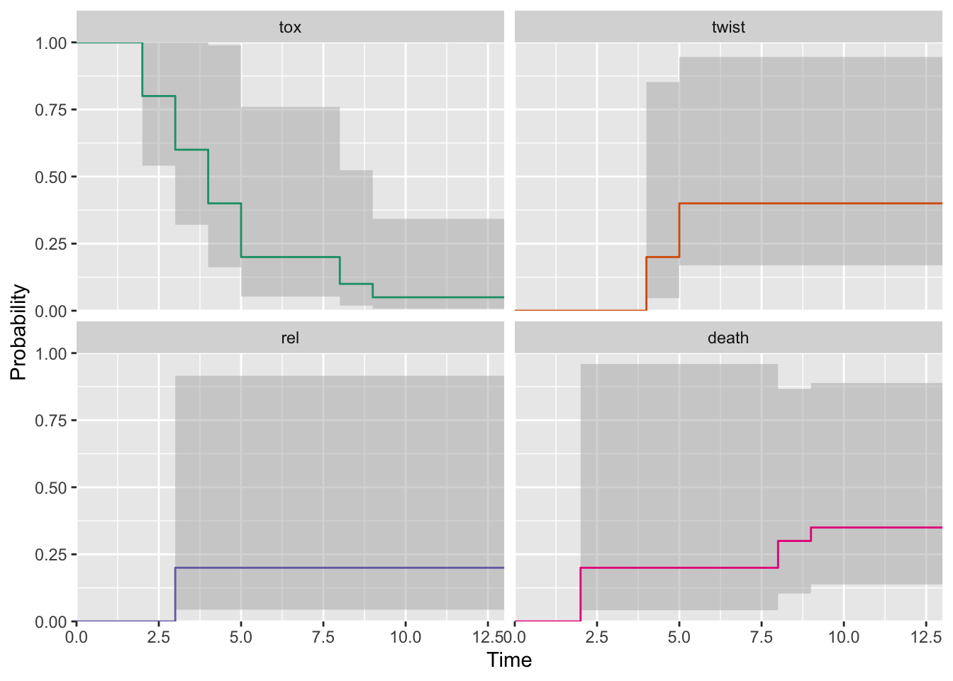
plot(p_model, use.ggplot = TRUE, type = 'separate', conf.int = 0.95,conf.type = 'log')