SIR-like model with deSolve in deterministic and stochastic version

Summary

Here, an model based on the SIR model is presented in a deterministic version and in a non-deterministic version. For solving the ODEs (deterministic version) and the stochastic difference equations (stochastic version), the R package deSolve is used.

Defining and solving a simple ODE model

A simplified SIR model: $$\frac{dS}{dt}=-\frac{\beta IS}{N}$$

$$\frac{dI}{dt}=\frac{\beta IS}{N}-\gamma I$$

$$\frac{dR}{dt}=\gamma I$$

Loading the required libraries and defining utility functions

library('ggplot2')
library('tidyverse')
library('deSolve')
theme_set(theme_bw())

plot_deSolve_result <- function(result) {
  tib <- as_tibble(unclass(result))  
  vars <- colnames(result)[-1]
  long <- pivot_longer(tib, cols = all_of(vars))
  long$name <- factor(long$name, levels = c('S', 'I', 'R'))
  ggplot(long, aes(time, value, colour = name)) + 
    geom_line() + 
    labs(colour = 'Compartment', 
         x = 'Time',
         y = 'Fraction')
}

Definition of the parameters

parameters <- list(beta = 0.2, 
                   gamma = .01,
                   lambda = 0)

infected_initial <- 0.01
initial_condition <- 
  c(S = 1 - infected_initial,
    I = infected_initial,
    R = 0)

t_max <- 100
step_length <- t_max / 100
timepoints <- seq(0, 150, length.out = 100)

Deterministic model

sir_ode_deterministic <- function(t, state, pars) {
  with(as.list(c(state, pars)), {
    dS <- - beta * I * S + lambda * R
    dI <- beta * I * S - gamma * I
    dR <- gamma * I - lambda * R
    return(list(c(dS = dS, dI = dI, dR = dR)))
  }) 
}


sir_solution_deterministic <- 
  ode(y = initial_condition, 
      times = timepoints,
      func = sir_ode_deterministic,
      parms = parameters)
plot_deSolve_result(sir_solution_deterministic)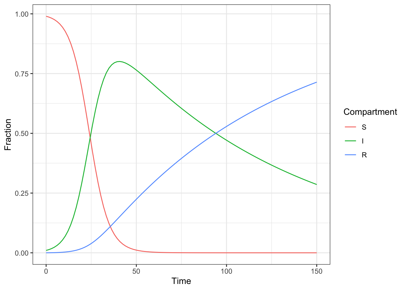

Stochastic model

sir_ode_stochastic <- function(t, state, pars) {
  with(as.list(c(state, pars)), {
    S_new <- S - beta * I * S * step_length
    I_new <- I + (beta * I * S - gamma * I) * step_length
    R_new <- R + gamma * I * step_length
    
    new_values <-c(S = S_new, I = I_new, R = R_new)
    new_values <- new_values * rlnorm(3, meanlog = 0, sdlog = 0.05)
    new_values <- new_values / sum(new_values)
    return(list(new_values))
  })
}

sir_solution_stochastic <- 
  ode(y = initial_condition, 
      times = timepoints,
      func = sir_ode_stochastic,
      parms = parameters, 
      method = 'iteration')

plot_deSolve_result(sir_solution_stochastic)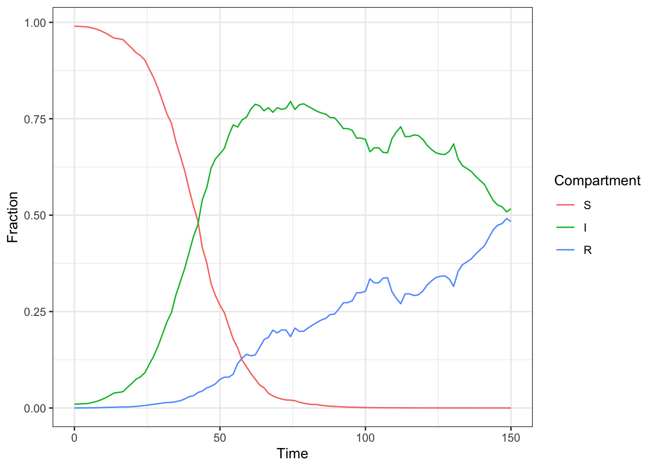

Conclusion

The R package deSolve can be used to solve deterministic ODEs and stochastic difference equations.