Latent profile analysis – second post

Published

August 27, 2026

library('tidyLPA')
library('tidyverse')

# Example data with four numeric variables
set.seed(123)

dat <- tibble(
  x1 = rnorm(200),
  x2 = rnorm(200),
  x3 = rnorm(200),
  x4 = rnorm(200)
)

# Standardization is often useful
dat_z <- dat

# Fit models with 1-4 latent profiles
models <- dat_z |>
  estimate_profiles(1:10)

Warning: 
One or more analyses resulted in warnings! Examine these analyses carefully: model_1_class_7, model_1_class_8, model_1_class_9, model_1_class_10

# Compare models
get_fit(models)

# A tibble: 10 × 20
   Model Classes LogLik parameters     n   AIC   AWE   BIC  CAIC   CLC   KIC
   <dbl>   <int>  <dbl>      <dbl> <int> <dbl> <dbl> <dbl> <dbl> <dbl> <dbl>
 1     1       1 -1118.          8   200 2253. 2343. 2279. 2287. 2239. 2264.
 2     1       2 -1118.         13   200 2261. 2411. 2304. 2317. 2236. 2277.
 3     1       3 -1109.         18   200 2254. 2462. 2313. 2331. 2219. 2275.
 4     1       4 -1108.         23   200 2262. 2527. 2337. 2360. 2217. 2288.
 5     1       5 -1105.         28   200 2265. 2589. 2358. 2386. 2210. 2296.
 6     1       6 -1104.         33   200 2273. 2655. 2382. 2415. 2208. 2309.
 7     1       7 -1099.         38   200 2274. 2714. 2400. 2438. 2200. 2315.
 8     1       8 -1095.         43   200 2276. 2773. 2418. 2461. 2191. 2322.
 9     1       9 -1094.         48   200 2285. 2840. 2443. 2491. 2190. 2336.
10     1      10 -1094.         53   200 2293. 2907. 2468. 2521. 2189. 2349.
# ℹ 9 more variables: SABIC <dbl>, ICL <dbl>, Entropy <dbl>, prob_min <dbl>,
#   prob_max <dbl>, n_min <dbl>, n_max <dbl>, BLRT_val <dbl>, BLRT_p <dbl>

plot(models)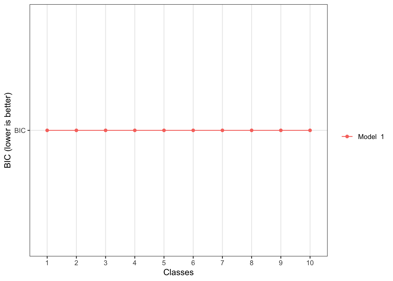

# vignette('Introduction_to_tidyLPA', package = 'tidyLPA')

n <- 1000

dat <- tibble(
  x1 = c(rnorm(n, 0), rnorm(n, 5), rnorm(n, 10)),
  x2 = c(rnorm(n, 3), rnorm(n, 0), rnorm(n, 3))
)

dat |> 
  ggplot(aes(x1, x2, alpha = 0.2)) + geom_point()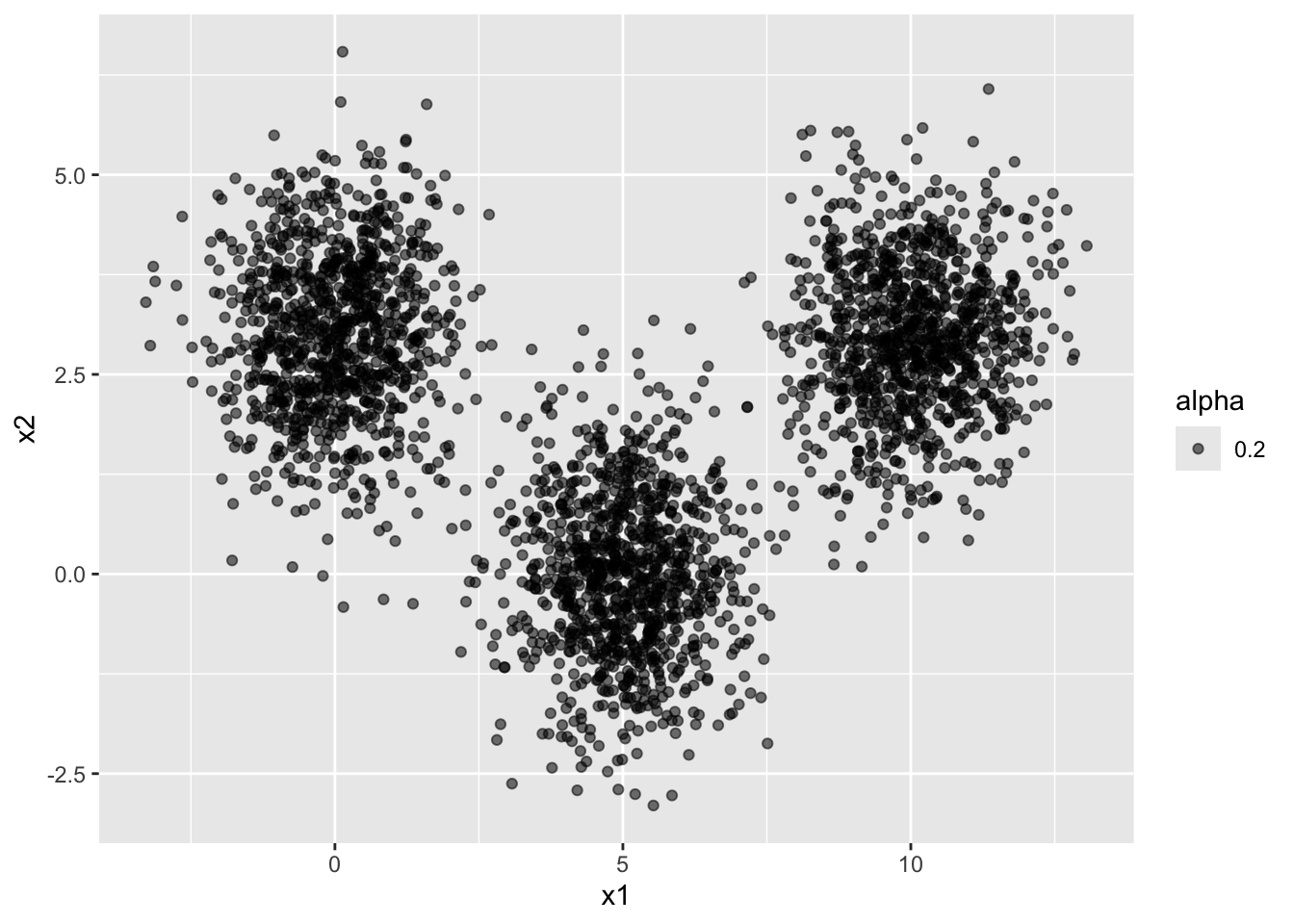

models <- dat |> 
  estimate_profiles(1:10)

Warning: 
One or more analyses resulted in warnings! Examine these analyses carefully: model_1_class_10

get_fit(models)

# A tibble: 10 × 20
   Model Classes  LogLik parameters     n    AIC    AWE    BIC   CAIC    CLC
   <dbl>   <int>   <dbl>      <dbl> <int>  <dbl>  <dbl>  <dbl>  <dbl>  <dbl>
 1     1       1 -14496.          4  3000 28999. 29065. 29023. 29027. 28993.
 2     1       2 -14182.          7  3000 28378. 28496. 28420. 28427. 28366.
 3     1       3 -11826.         10  3000 23671. 23840. 23731. 23741. 23653.
 4     1       4 -11825.         13  3000 23676. 23896. 23754. 23767. 23652.
 5     1       5 -11822.         16  3000 23676. 23946. 23772. 23788. 23645.
 6     1       6 -11820.         19  3000 23677. 23999. 23791. 23810. 23641.
 7     1       7 -11817.         22  3000 23678. 24051. 23810. 23832. 23635.
 8     1       8 -11818.         25  3000 23687. 24111. 23837. 23862. 23638.
 9     1       9 -11818.         28  3000 23693. 24168. 23861. 23889. 23638.
10     1      10 -11817.         31  3000 23696. 24222. 23882. 23913. 23635.
# ℹ 10 more variables: KIC <dbl>, SABIC <dbl>, ICL <dbl>, Entropy <dbl>,
#   prob_min <dbl>, prob_max <dbl>, n_min <dbl>, n_max <dbl>, BLRT_val <dbl>,
#   BLRT_p <dbl>