Ornstein Uhlenbeck

library('tidyverse')
library('sde')

sim_ou <- function(timepoints, x0, theta) {
  timepoints <- c(0, timepoints)
  dT <- diff(timepoints)
  X <- numeric(length(timepoints))
  X[1] <- x0
  for(i in 2:length(timepoints)) {
    X[i] <- rcOU(1, dT[i - 1], X[i - 1], theta)
  }
  return(tibble(timepoints, X))
}

n <- 30000
Theta <- c(0, 0.17, 1.3)
rr <- sim_ou(sort(runif(n, 0, n)), 0, theta = Theta); plot(rr$timepoints, rr$X)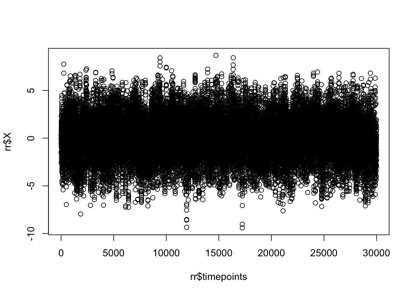

p_ou <- function(rr, theta) {
  x <- rr$X[-1]
  x0 <- rr$X[-nrow(rr)]
  Dt <- diff(rr$timepoints)
  pcOU(x, Dt, x0, theta)
}



pp <- p_ou(rr, Theta)
plot(pp)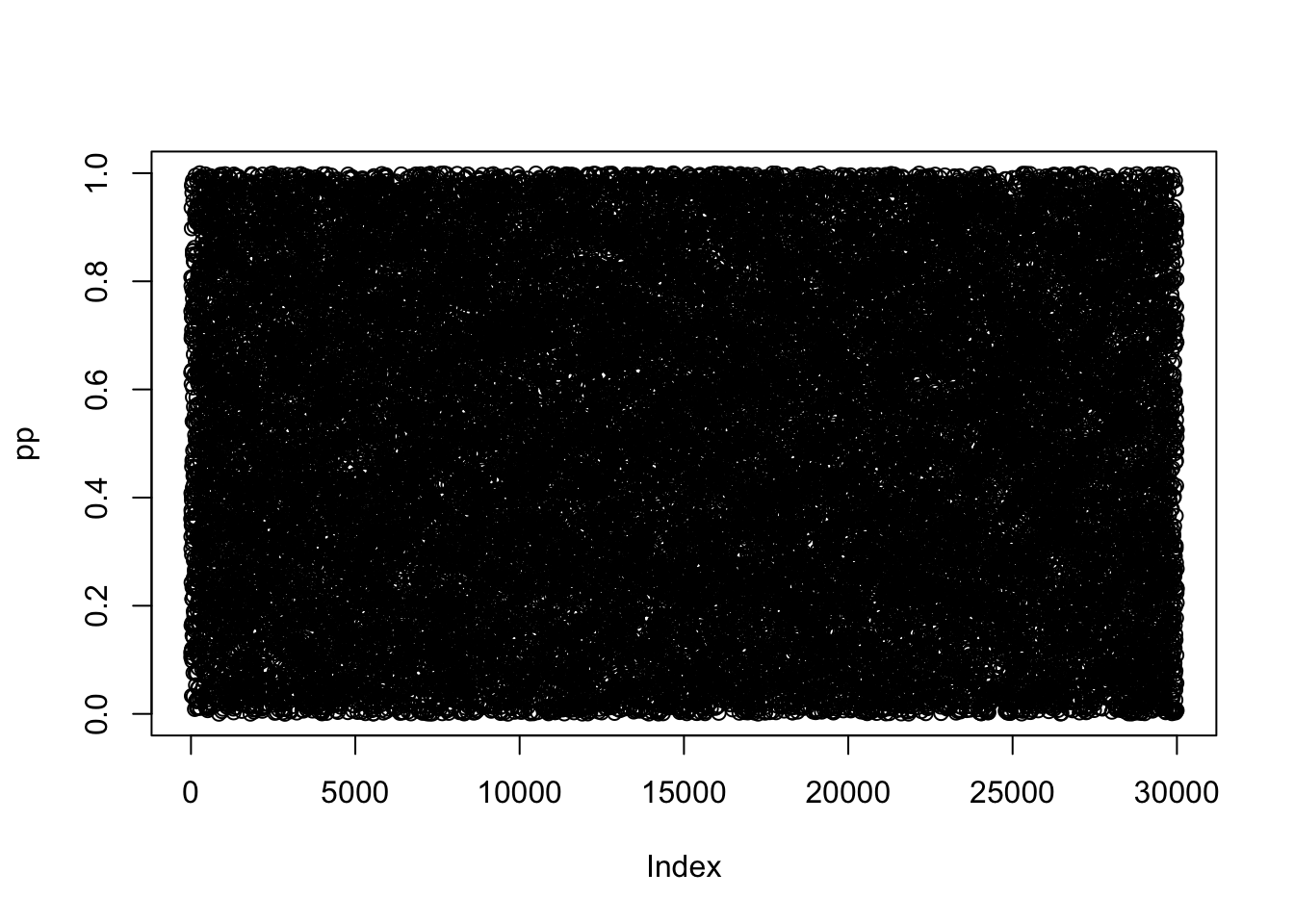

plot(ecdf(pp))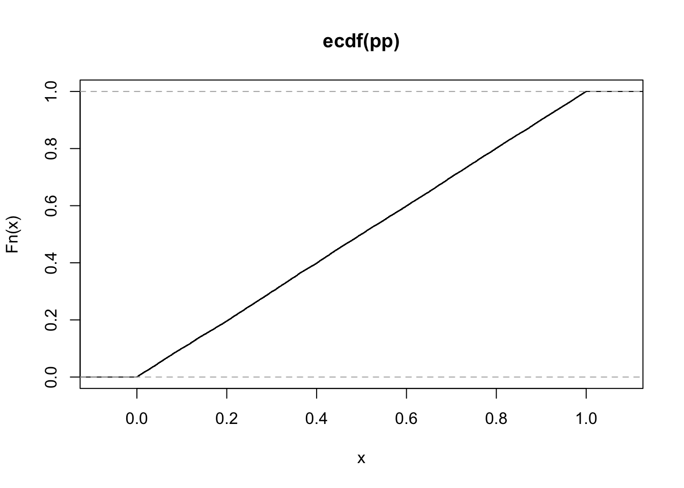

ll_ou <- function(rr, theta) {
  x <- rr$X[-1]
  x0 <- rr$X[-nrow(rr)]
  Dt <- diff(rr$timepoints)
  dcOU(x, Dt, x0, theta, log = TRUE) |> sum()
}

ll_ou(rr, Theta)

[1] -39438.25

bb <- optim(c(1, 1), function(p) {
  Theta <- c(0, exp(p[1]), exp(p[2]))
  -ll_ou(rr, Theta)
} )

exp(bb$par)

[1] 0.1673832 1.2961883