library(tidyverse)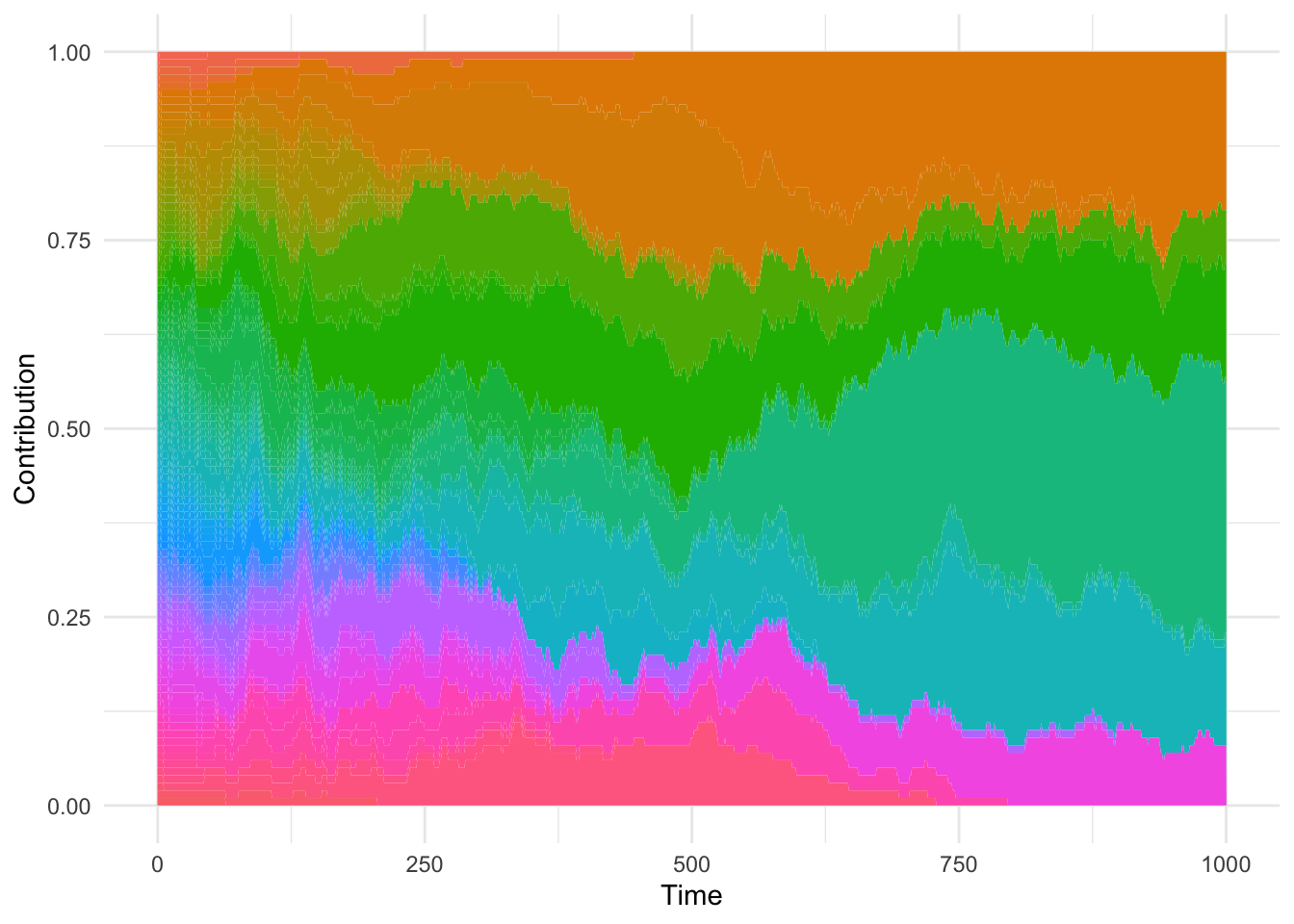
set.seed(1)Moran process
R
What causes clinical symptoms in hematological malignancies?
- Malignant clone outcompetes own cell type
- Malignant clone outcompetes other needed cell types
- Malignant clone causes inflammation
- Malignant clone does other “bad” things (what?)
- ???
Measuring invasiveness
- Can we disentangle expansion in “own” niche vs. expansion in niches of other cell types?
- Generally:
- First mutations lead to mutation in “own” niche
- Later mutations lead to invasion in other niches
Can level of invasion be quantified with available data?
Model sketch
- Two compartments
- Compartment A, from which cancer arises
- Compartment B, that is an “umbrella compartment” for all other hematopoietic cells
- A and B contain \(n_A\) and \(n_B\) cells
- Each time step, one cell dies and cell divides
- Two phases:
- Non-invasive expansion: Clone has increased probability to divide within A only
- Invasive expansion: Clone can now enter also compartment B
Can this model be fitted to mutation trees and blood count data?
What would we learn?
- Formal way to estimate invasive potential of new mutations
Additional aspect
- More efficient utilization of niche resources
- Asymptotically: Growth independent of niche
Background
Simulation
simulate_moran <- function(n, t_max, record_at) {
  current_state <- 1:n
  contribution <- tibble()
  i <- 0 # time counter
  j <- 1 # recording counter
  while(i <= t_max & length(unique(current_state)) > 1) {
    if(record_at[j] == i) {
      clone_sizes <- tabulate(current_state, nbins = n) / n
      contribution <-
        bind_rows(
          contribution,
          tibble(time = i,
                 id = paste0('c', 1:n),
                 size = clone_sizes))
      j <- j + 1
    }
    ii_death <- sample.int(n, 1)
    ii_birth <- sample.int(n, 1)
    current_state[ii_death] <- current_state[ii_birth]
    i <- i + 1
  }
  return(list(clonal_conversion_time = i,
              contribution = contribution))
}

log_sim_length <- 10
t_max <- 2^log_sim_length
record_at <- c(2^(0:log_sim_length))
record_at <- c(0:1000, 10000)

result <- simulate_moran(n = 100, t_max = t_max, record_at = record_at)

result$contribution |>
  ggplot(aes(time, size, fill = id)) +
  geom_area() +
  theme_minimal() +
  theme(legend.position="none") +
  labs(x = 'Time', y = 'Contribution')