Bivariate dataset - linear regression and neural net

Basic neural net

Init

set.seed(1)
library('neuralnet')
library('tidyverse')
library('knitr')

We are looking at the cars dataset (more about the dataset via help(cars))

• dist is the stopping distance (not what I said today)

cars |> 
  ggplot(aes(dist, speed)) + 
  geom_point()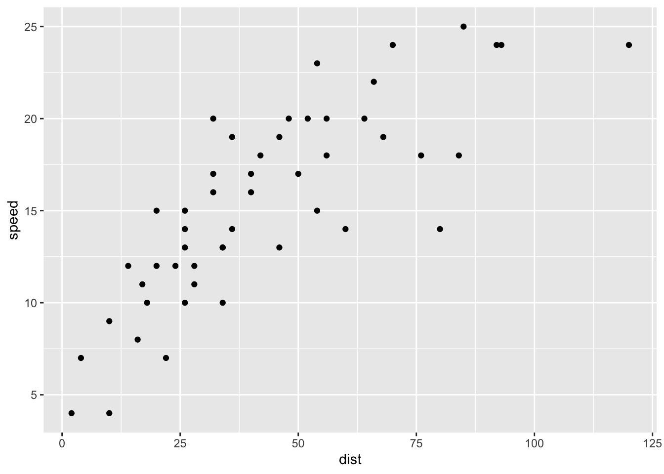

We can fit a linear regression model:

fm_lm <- lm(speed ~ dist, data = cars)
summary(fm_lm)

Call:
lm(formula = speed ~ dist, data = cars)

Residuals:
    Min      1Q  Median      3Q     Max 
-7.5293 -2.1550  0.3615  2.4377  6.4179 

Coefficients:
            Estimate Std. Error t value Pr(>|t|)    
(Intercept)  8.28391    0.87438   9.474 1.44e-12 ***
dist         0.16557    0.01749   9.464 1.49e-12 ***
---
Signif. codes:  0 '***' 0.001 '**' 0.01 '*' 0.05 '.' 0.1 ' ' 1

Residual standard error: 3.156 on 48 degrees of freedom
Multiple R-squared:  0.6511,    Adjusted R-squared:  0.6438 
F-statistic: 89.57 on 1 and 48 DF,  p-value: 1.49e-12

We can do basically the same thing using a neural net with a single perceptron

• Note that the coefficients of the linear regression model are (almost) identical to the weights in the neural net

nn_0 <- neuralnet(speed ~ dist, 
                  linear.output = TRUE, 
                  data = cars, 
                  hidden = 0)
plot(nn_0, rep = 'best')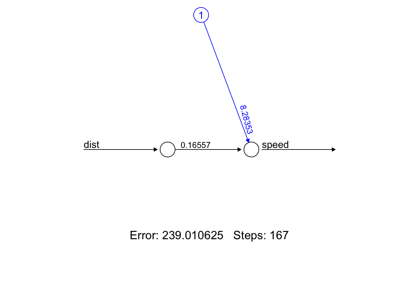

The neuralnet package uses RSS / 2 as cost function (this might be the reason)

# RSS / 2 of the linear regression model
sum(((predict(fm_lm) - cars$speed))^2) / 2

[1] 239.0106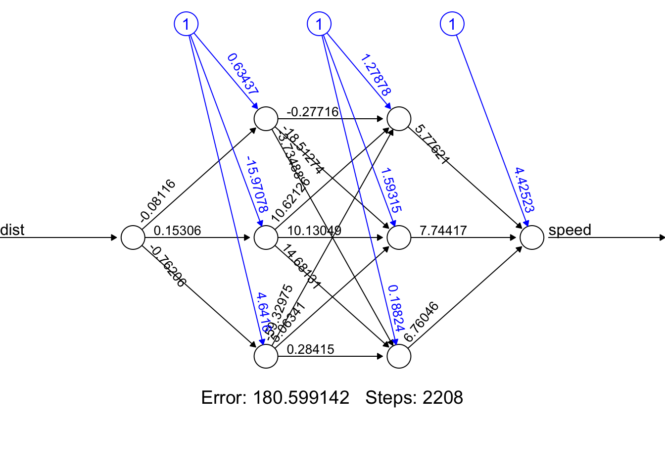

A more complex neural net can be trained (two hidden layers with three perceptrons each):

• stepmax and threshold have to be tuned due to problems with convergence

nn_1 <- neuralnet(speed ~ dist, 
                  linear.output = TRUE, data = cars, 
                  hidden = c(3, 3), 
                  stepmax = 1e+7, threshold = .5)

plot(nn_1, rep = 'best')

The predictions of the simple (basically linear regression) neural net and the more complex neural net plotted here:

cc <- cars |> mutate(
  nn_0_prediction = as.vector(predict(nn_0, cars)),
  nn_1_prediction = as.vector(predict(nn_1, cars))) |> 
  pivot_longer(cols = c(nn_0_prediction, nn_1_prediction))  

cc |> 
  ggplot(aes(dist, value, color = name)) + geom_line(linewidth = 2) + 
  geom_point(aes(dist, speed, color = 'original data'), data = cars) +
  labs(y = 'speed', color = 'Group')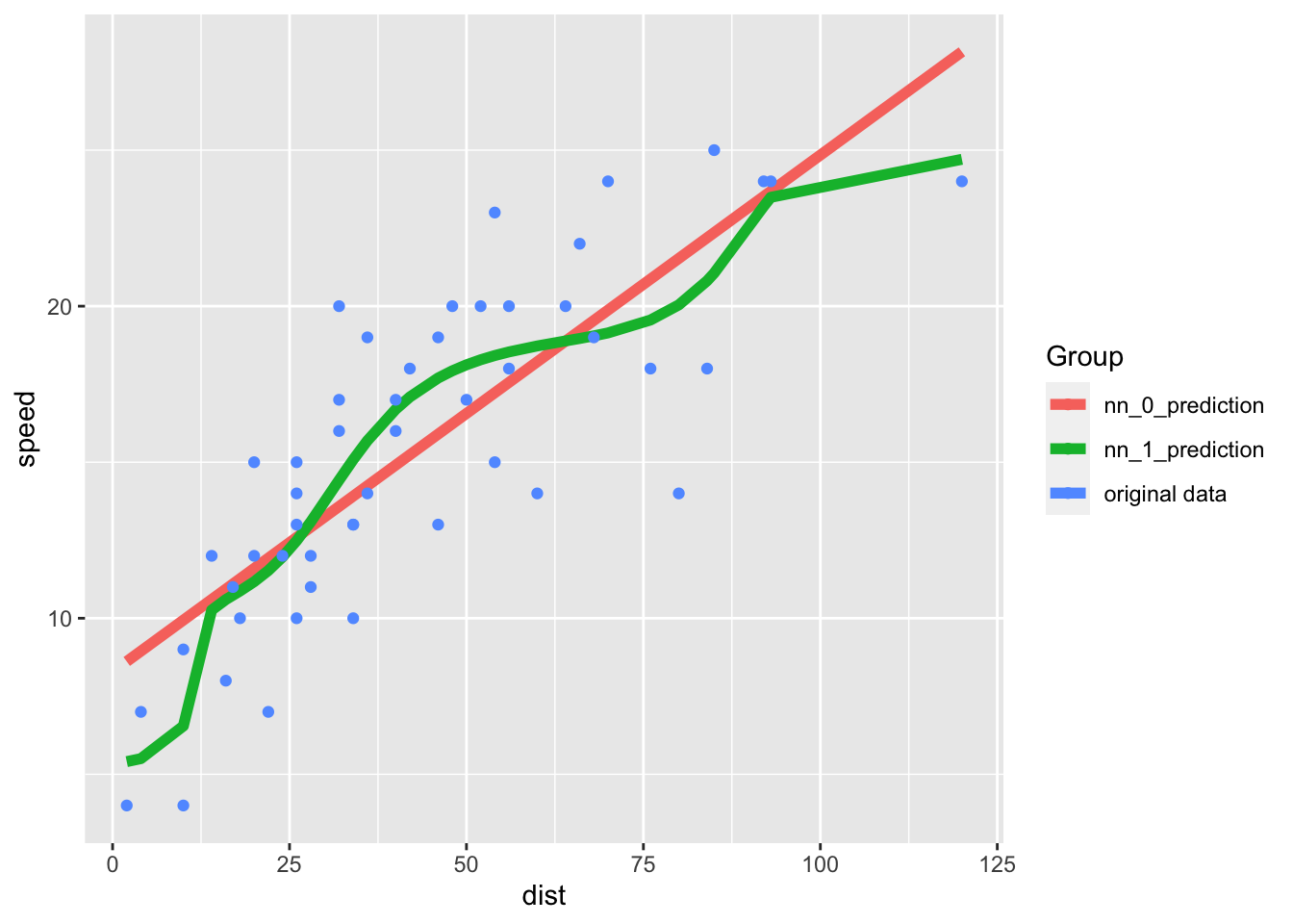

The residual sum of squares is (as expected) less in the more complex model:

cc |> 
  group_by(name) |> 
  summarize(RSS = sum((value - speed)^2)) |> 
  kable(align = 'c', digits = 2)

name	RSS
nn_0_prediction	478.02
nn_1_prediction	361.20