Leo’s project

Part 1: Simulating data

Background

In hematological cancers, blood stem cells can be transferred to a patient after chemothery. The blood stem cells may proliferate in the patient and populate the patient’s peripheral blood afterwards.

Chimerism is defined as the ratio of the number of blood cells originating from the transplanted cells and the total number of blood cells in the patient’s blood.

Here, a sigmoidal model for the temporal development of chimerism after transplantion is introduced and in silico data are simulated.

Leo also posted a question about this model on the STAN forum: https://discourse.mc-stan.org/t/bad-diagnostics-with-multilevel-models/29091?u=leonhardschwager

Initialization

library('tidyverse')
set.seed(1)

Definition of model function to predict chimerism

• Source: https://en.wikipedia.org/wiki/Logistic_function

calc_chimerism <- function(day, d = 1, b = 1, e = 5) {
# day: for which day the chimerism shall be calculated
# d: maximum value of the curve
# b: the logistic growth rate or steepness of the curve
# e:  location of the midpoint of the sigmoid function
  d / (1 + exp(-b * (day - e)))
}

# plot the function with default values:
ggplot() + stat_function(fun = calc_chimerism) + 
  xlim(0, 10) + labs(x = 'Time', y = 'Chimerism')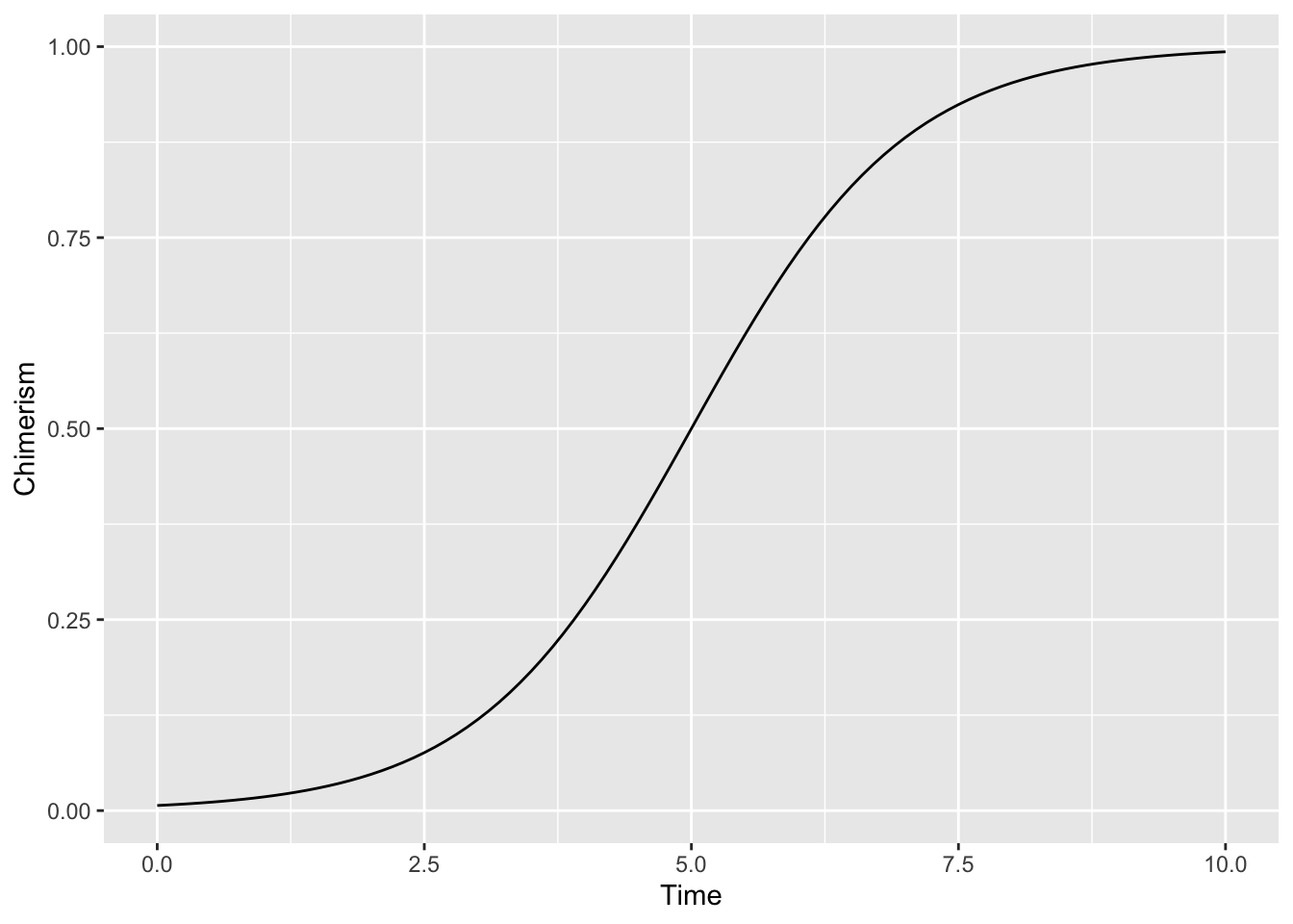

Set parameters

nr_of_patients <- 10
nr_of_measurements <- 10 # per patient
d <- runif(n = nr_of_patients, min = 0.6, max = 1)
b <- rnorm(n = nr_of_patients, mean = 1, sd = 0.1)
e <- runif(n = nr_of_patients, min = 5, max = 15)

Construct independent values

dat <- tibble(patient_id = factor(1:nr_of_patients), 
              d = d, 
              b = b, 
              e = e) %>%
  expand_grid(measurement = 1:nr_of_measurements)

# compute timepoints symetrical equidistant 
# in both directions of the sigmoid midpoint 
# of the curve:
dat$day <- dat$e * 2 * dat$measurement / nr_of_measurements

Apply model function to calculate dependendant values

dat$chimerism <- calc_chimerism(day = dat$day, 
                                d = dat$d, 
                                b = dat$b, 
                                e = dat$e)

Plot the simulated data

ggplot(dat, aes(day, chimerism)) + 
  geom_point() + geom_line() + 
  facet_wrap(~ patient_id, ncol = 3, scales = 'free_x') + 
  xlim(0, NA) + ylim(0, 1)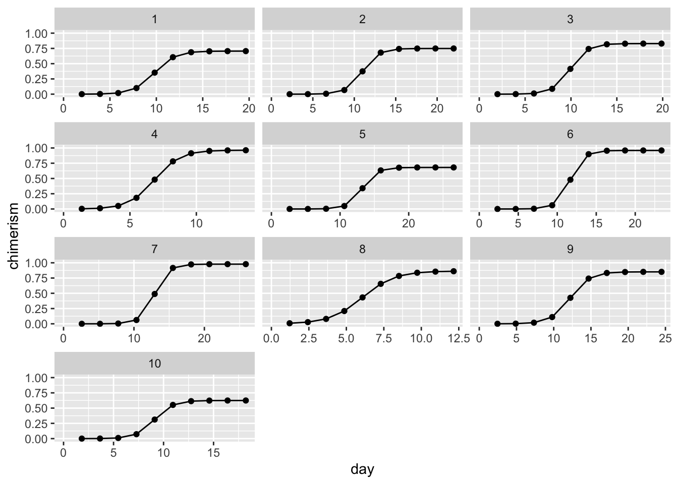

ggplot(dat, aes(day, chimerism, color = patient_id)) + 
  geom_point() + geom_line() + 
  ylim(0, 1)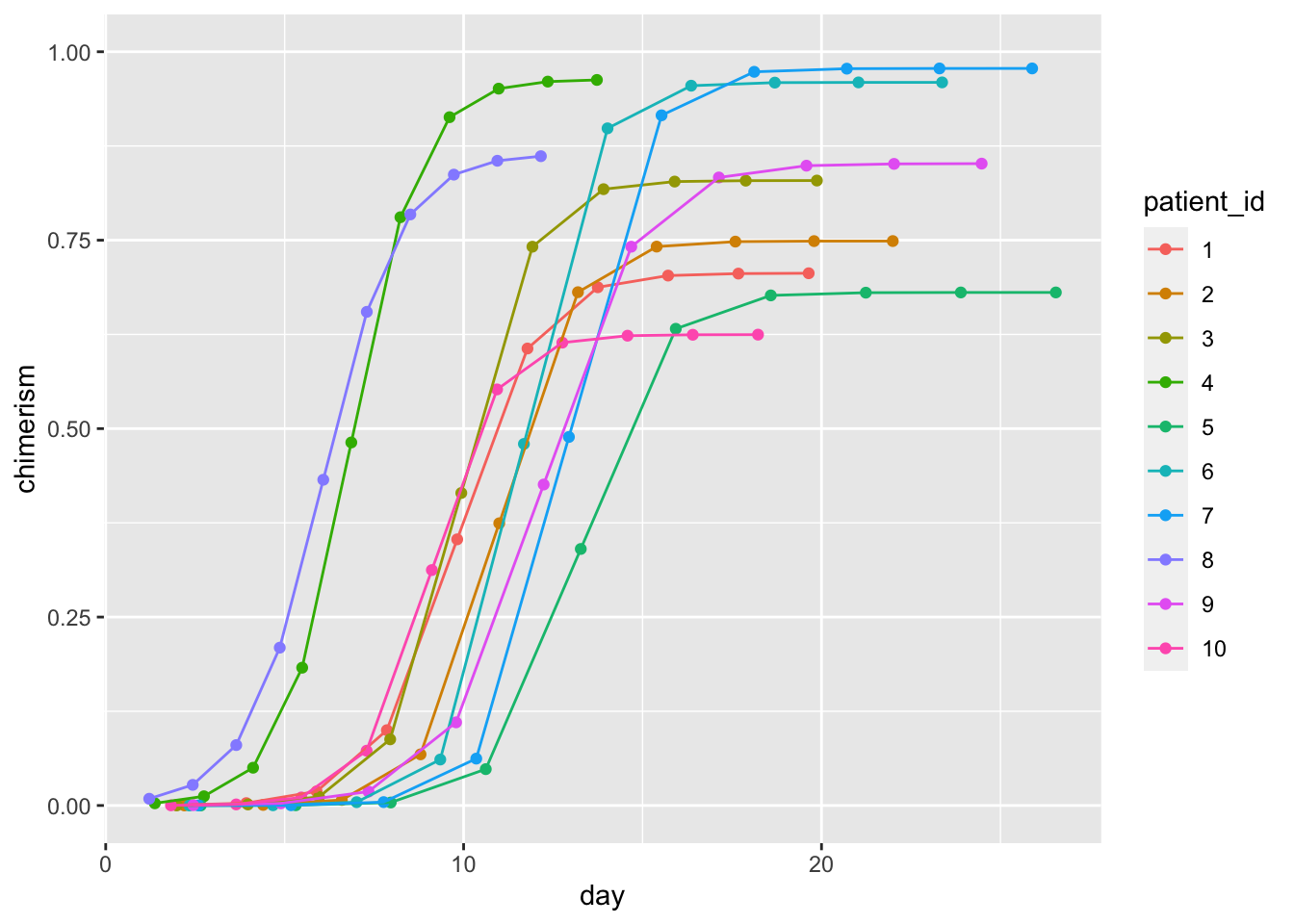

Conclusion

Part 2: Fitting models

Fitting a simple model

library('brms')

Loading required package: Rcpp

Loading 'brms' package (version 2.19.0). Useful instructions
can be found by typing help('brms'). A more detailed introduction
to the package is available through vignette('brms_overview').

Attaching package: 'brms'

The following object is masked from 'package:stats':

    ar

# help(package = 'brms')
# prior1 <- prior(normal(1, 0.1), nlpar = ')